Density matrix plot

An intuitive way to look at eigenstates is to plot the charge density. For multi-electron wave-functions one can not plot the wave-function (it depends on $3\times n$ coordinates) but the charge density is a well defined simple quantity. We here use the rendering options of \textit{Mathematica} in combination with the package for \textit{Mathematica} (Quanty.nb) to plot the density matrix of the lowest three eigenstates in NiO.

density_matrix_plots_Mathematica.Quanty

-- It is often nice to make plots of the resulting "wave-functions" Now one can not
-- simply plot a multi-electron wavefunction \psi(r_1,r_2,r_3, ..., r_n) as it depends
-- on 3n coordinates.
-- One can plot the resulting charge density.
 
-- This example calculates the density matrix of a state and then calls Mathematica to
-- make a density plot of this matrix.
 
-- the script for mathematica is included in the input file
-- the input string needs calculated data which will be substituted before calling mathematica
 
-- You need to change the absolute path in the script below
mathematicaInput = [[
Needs["Quanty`PlotTools`"];
rho=%s;
pl = Table[ Rasterize[ DensityMatrixPlot[IdentityMatrix[10] - rho[ [i] ], PlotRange -> {{-0.4, 0.4}, {-0.4, 0.4}, {-0.4, 0.4}}] ], {i, 1, Length[rho]}];
For[i = 1, i <= Length[pl], i++,
    Export["/Users/haverkort/Documents/Quanty/Example_and_Testing/History/current/Tutorials/40_NiO_Ligand_Field/Rho" <> ToString[i] <> ".png", pl[ [i] ] ];
   ];
Quit[];
]]
 
-- We use the definitions of all operators and basis orbitals as defined in the file
-- include and can afterwards directly continue by creating the Hamiltonian
-- and calculating the spectra
 
dofile("Include.Quanty")
 
-- The parameters and scheme needed only includes the ground-state (d^8) configuration
 
-- We follow the energy definitions as introduced in the group of G.A. Sawatzky (Groningen)
-- J. Zaanen, G.A. Sawatzky, and J.W. Allen PRL 55, 418 (1985)
-- for parameters of specific materials see
-- A.E. Bockquet et al. PRB 55, 1161 (1996)
-- After some initial discussion the energies U and Delta refer to the center of a configuration
-- The L^10 d^n   configuration has an energy 0
-- The L^9  d^n+1 configuration has an energy Delta
-- The L^8  d^n+2 configuration has an energy 2*Delta+Udd
--
-- If we relate this to the onsite energy of the L and d orbitals we find
-- 10 eL +  n    ed + n(n-1)     U/2 == 0
--  9 eL + (n+1) ed + (n+1)n     U/2 == Delta
--  8 eL + (n+2) ed + (n+1)(n+2) U/2 == 2*Delta+U
-- 3 equations with 2 unknowns, but with interdependence yield:
-- ed = (10*Delta-nd*(19+nd)*U/2)/(10+nd)
-- eL = nd*((1+nd)*Udd/2-Delta)/(10+nd)
-- 
-- note that ed-ep = Delta - nd * U and not Delta
-- note furthermore that ep and ed here are defined for the onsite energy if the system had
-- locally nd electrons in the d-shell. In DFT or Hartree Fock the d occupation is in the end not
-- nd and thus the onsite energy of the Kohn-Sham orbitals is not equal to ep and ed in model
-- calculations.
--
-- note furthermore that ep and eL actually should be different for most systems. We happily ignore this fact
-- 
-- We normally take U and Delta as experimentally determined parameters
 
-- number of electrons (formal valence)
nd = 8
-- parameters from experiment (core level PES)
Udd     =  7.3
Delta   =  4.7
-- parameters obtained from DFT (PRB 85, 165113 (2012))
F2dd    = 11.14 
F4dd    =  6.87
F2pd    =  6.67
tenDq   =  0.56
tenDqL  =  1.44
Veg     =  2.06
Vt2g    =  1.21
zeta_3d =  0.081
Bz      =  0.000001
H112    =  0.120
 
ed      = (10*Delta-nd*(19+nd)*Udd/2)/(10+nd)
eL      = nd*((1+nd)*Udd/2-Delta)/(10+nd)
 
F0dd    = Udd + (F2dd+F4dd) * 2/63
 
Hamiltonian =  F0dd*OppF0_3d + F2dd*OppF2_3d + F4dd*OppF4_3d + zeta_3d*Oppldots_3d + Bz*(2*OppSz_3d + OppLz_3d) + H112 * (OppSx_3d+OppSy_3d+2*OppSz_3d)/sqrt(6) + tenDq*OpptenDq_3d + tenDqL*OpptenDq_Ld + Veg * OppVeg + Vt2g * OppVt2g + ed * OppN_3d + eL * OppN_Ld
 
-- we now can create the lowest Npsi eigenstates:
Npsi=3
-- in order to make sure we have a filling of 8 electrons we need to define some restrictions
StartRestrictions = {NF, NB, {"000000 00 1111111111 0000000000",8,8}, {"111111 11 0000000000 1111111111",18,18}}
 
psiList = Eigensystem(Hamiltonian, StartRestrictions, Npsi)
oppList={Hamiltonian, OppSsqr, OppLsqr, OppJsqr, OppSx_3d, OppLx_3d, OppSy_3d, OppLy_3d, OppSz_3d, OppLz_3d, Oppldots_3d, OppF2_3d, OppF4_3d, OppNeg_3d, OppNt2g_3d, OppNeg_Ld, OppNt2g_Ld, OppN_3d}
 
-- print of some expectation values
print("  #    <E>      <S^2>    <L^2>    <J^2>    <S_x^3d> <L_x^3d> <S_y^3d> <L_y^3d> <S_z^3d> <L_z^3d> <l.s>    <F[2]>   <F[4]>   <Neg^3d> <Nt2g^3d><Neg^Ld> <Nt2g^Ld><N^3d>");
for i = 1,#psiList do
  io.write(string.format("%3i ",i))
  for j = 1,#oppList do
    expectationvalue = Chop(psiList[i]*oppList[j]*psiList[i])
    io.write(string.format("%8.3f ",expectationvalue))
  end
  io.write("\n")
end
io:flush()
 
-- we now make plots of the charge density
 
function tableToMathematica(t)
  local ret = "{ "
  for k,v in pairs(t) do
    if k~=1 then 
      ret = ret.." , "
    end
    if (type(v) == "table") then
      ret = ret..tableToMathematica(v)
    else
      ret = ret..string.format("%18.15f + (%18.15f) I ",Complex.Re(v),Complex.Im(v))
    end
  end
  ret = ret.." }"
  return ret
end
 
-- the d-orbitals are found at position 8 to 17 (see the include file)
rhoList = DensityMatrix(psiList, {8,9,10,11,12,13,14,15,16,17})
rhoListMathematicaForm = tableToMathematica(rhoList)
 
file = io.open("densitymatrix.nb", "w")
file:write( mathematicaInput:format( rhoListMathematicaForm ) )
file:close()
 
os.execute("/Applications/Mathematica08.app/Contents/MacOS/MathKernel -run '<<densitymatrix.nb'")
os.execute("convert Rho1.png -transparent white temp.png ; convert temp.png Rho1.eps ; rm temp.png")
os.execute("convert Rho2.png -transparent white temp.png ; convert temp.png Rho2.eps ; rm temp.png")
os.execute("convert Rho3.png -transparent white temp.png ; convert temp.png Rho3.eps ; rm temp.png")

$S_z=-1$	$S_z=0$	$S_z=1$
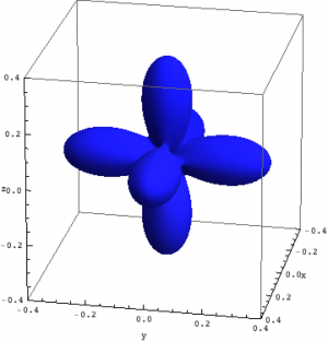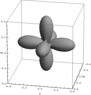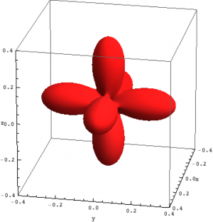Hole density of the $3d$ Ni orbitals in NiO

The plots can be seen in Fig. \ref{figNiODensityMatrix}. We show the hole density (identity matrix minus the density matrix) which has lobes towards the O atoms. Ni in NiO has a hole in the $x^2-y^2$ and in the $z^2$ orbital. The color represent the spin down, $S_z=0$ and spin up state of the lowest triplet.

The output to the screen is:

Density_matrix_plots_Mathematica.out

  #    <E>      <S^2>    <L^2>    <J^2>    <S_x^3d> <L_x^3d> <S_y^3d> <L_y^3d> <S_z^3d> <L_z^3d> <l.s>    <F[2]>   <F[4]>   <Neg^3d> <Nt2g^3d><Neg^Ld> <Nt2g^Ld><N^3d>
  1   -3.503    1.999   12.000   15.095   -0.370   -0.115   -0.370   -0.115   -0.741   -0.230   -0.305   -1.042   -0.924    2.186    5.990    3.825    6.000    8.175 
  2   -3.395    1.999   12.000   15.160   -0.002   -0.000   -0.002   -0.000   -0.003   -0.001   -0.322   -1.043   -0.925    2.189    5.988    3.823    6.000    8.178 
  3   -3.286    1.999   12.000   15.211    0.369    0.113    0.369    0.113    0.737    0.227   -0.336   -1.043   -0.925    2.193    5.987    3.820    6.000    8.180 
Mathematica 8.0 for Mac OS X x86 (64-bit)
Copyright 1988-2011 Wolfram Research, Inc.
Loaded the Quanty : Plot Tools Package - version 2016.4.13
Written by Maurits W. Haverkort