RIXS $L_{2,3}M_{4,5}$

Using the function ResonantSpectra we can calculate inelastic x-ray scattering. (or other second order processess) Here we show the example of $d$-$d$ excitations in NiO using RIXS. Due to an ever increasing resolution this method gains rapidly in popularity and impact. See for example the combined work of Ghiringhelli \textit{et al.} For NiO see \cite{Ghiringhelli:2005kp}.

A script to calculate these spectra is:

RIXS_L23M45.Quanty

-- this example calculates the resonant inelastic x-ray scattering in NiO we look at the
-- Ni L23M45 edge, i.e. we make an excitation from 2p to 3d (L23) and decay from the
-- 3d shell back to the 2p shell (final "hole" in the 3d shell M45 edge). These spectra
-- measure d-d excitations and or magnons.
 
-- We use the definitions of all operators and basis orbitals as defined in the file
-- 44_50_include and can afterwards directly continue by creating the Hamiltonian
-- and calculating the spectra
 
dofile("Include.Quanty")
 
-- The parameters and scheme needed is the same as the one used for XAS
 
-- We follow the energy definitions as introduced in the group of G.A. Sawatzky (Groningen)
-- J. Zaanen, G.A. Sawatzky, and J.W. Allen PRL 55, 418 (1985)
-- for parameters of specific materials see
-- A.E. Bockquet et al. PRB 55, 1161 (1996)
-- After some initial discussion the energies U and Delta refer to the center of a configuration
-- The L^10 d^n   configuration has an energy 0
-- The L^9  d^n+1 configuration has an energy Delta
-- The L^8  d^n+2 configuration has an energy 2*Delta+Udd
--
-- If we relate this to the onsite energy of the L and d orbitals we find
-- 10 eL +  n    ed + n(n-1)     U/2 == 0
--  9 eL + (n+1) ed + (n+1)n     U/2 == Delta
--  8 eL + (n+2) ed + (n+1)(n+2) U/2 == 2*Delta+U
-- 3 equations with 2 unknowns, but with interdependence yield:
-- ed = (10*Delta-nd*(19+nd)*U/2)/(10+nd)
-- eL = nd*((1+nd)*Udd/2-Delta)/(10+nd)
--
-- For the final state we/they defined
-- The 2p^5 L^10 d^n+1 configuration has an energy 0
-- The 2p^5 L^9  d^n+2 configuration has an energy Delta + Udd - Upd
-- The 2p^5 L^8  d^n+3 configuration has an energy 2*Delta + 3*Udd - 2*Upd
--
-- If we relate this to the onsite energy of the p and d orbitals we find
-- 6 ep + 10 eL +  n    ed + n(n-1)     Udd/2 + 6 n     Upd == 0
-- 6 ep +  9 eL + (n+1) ed + (n+1)n     Udd/2 + 6 (n+1) Upd == Delta
-- 6 ep +  8 eL + (n+2) ed + (n+1)(n+2) Udd/2 + 6 (n+2) Upd == 2*Delta+Udd
-- 5 ep + 10 eL + (n+1) ed + (n+1)(n)   Udd/2 + 5 (n+1) Upd == 0
-- 5 ep +  9 eL + (n+2) ed + (n+2)(n+1) Udd/2 + 5 (n+2) Upd == Delta+Udd-Upd
-- 5 ep +  8 eL + (n+3) ed + (n+3)(n+2) Udd/2 + 5 (n+3) Upd == 2*Delta+3*Udd-2*Upd
-- 6 equations with 3 unknowns, but with interdependence yield:
-- epfinal = (10*Delta + (1+nd)*(nd*Udd/2-(10+nd)*Upd) / (16+nd)
-- edfinal = (10*Delta - nd*(31+nd)*Udd/2-90*Upd) / (16+nd)
-- eLfinal = ((1+nd)*(nd*Udd/2+6*Upd)-(6+nd)*Delta) / (16+nd)
--
-- 
-- 
-- note that ed-ep = Delta - nd * U and not Delta
-- note furthermore that ep and ed here are defined for the onsite energy if the system had
-- locally nd electrons in the d-shell. In DFT or Hartree Fock the d occupation is in the end not
-- nd and thus the onsite energy of the Kohn-Sham orbitals is not equal to ep and ed in model
-- calculations.
--
-- note furthermore that ep and eL actually should be different for most systems. We happily ignore this fact
-- 
-- We normally take U and Delta as experimentally determined parameters
 
-- number of electrons (formal valence)
nd = 8
-- parameters from experiment (core level PES)
Udd     =  7.3
Upd     =  8.5
Delta   =  4.7
-- parameters obtained from DFT (PRB 85, 165113 (2012))
F2dd    = 11.14 
F4dd    =  6.87
F2pd    =  6.67
G1pd    =  4.92
G3pd    =  2.80
tenDq   =  0.56
tenDqL  =  1.44
Veg     =  2.06
Vt2g    =  1.21
zeta_3d =  0.081
zeta_2p = 11.51
Bz      =  0.000001
H112    =  0.120
 
ed      = (10*Delta-nd*(19+nd)*Udd/2)/(10+nd)
eL      = nd*((1+nd)*Udd/2-Delta)/(10+nd)
 
epfinal = (10*Delta + (1+nd)*(nd*Udd/2-(10+nd)*Upd)) / (16+nd)
edfinal = (10*Delta - nd*(31+nd)*Udd/2-90*Upd) / (16+nd)
eLfinal = ((1+nd)*(nd*Udd/2+6*Upd) - (6+nd)*Delta) / (16+nd)
 
F0dd    = Udd + (F2dd+F4dd) * 2/63
F0pd    = Upd + (1/15)*G1pd + (3/70)*G3pd
 
Hamiltonian =  F0dd*OppF0_3d + F2dd*OppF2_3d + F4dd*OppF4_3d + zeta_3d*Oppldots_3d + Bz*(2*OppSz_3d + OppLz_3d) + H112 * (OppSx_3d+OppSy_3d+2*OppSz_3d)/sqrt(6) + tenDq*OpptenDq_3d + tenDqL*OpptenDq_Ld + Veg * OppVeg + Vt2g * OppVt2g + ed * OppN_3d + eL * OppN_Ld
 
XASHamiltonian =  F0dd*OppF0_3d + F2dd*OppF2_3d + F4dd*OppF4_3d + zeta_3d*Oppldots_3d + Bz*(2*OppSz_3d + OppLz_3d)+ H112 * (OppSx_3d+OppSy_3d+2*OppSz_3d)/sqrt(6) + tenDq*OpptenDq_3d + tenDqL*OpptenDq_Ld + Veg * OppVeg + Vt2g * OppVt2g + edfinal * OppN_3d + eLfinal * OppN_Ld + epfinal * OppN_2p + zeta_2p * Oppcldots + F0pd * OppUpdF0 + F2pd * OppUpdF2 + G1pd * OppUpdG1 + G3pd * OppUpdG3  
 
-- we now can create the lowest Npsi eigenstates:
Npsi=3
-- in order to make sure we have a filling of 8 electrons we need to define some restrictions
StartRestrictions = {NF, NB, {"000000 00 1111111111 0000000000",8,8}, {"111111 11 0000000000 1111111111",18,18}}
 
psiList = Eigensystem(Hamiltonian, StartRestrictions, Npsi)
oppList={Hamiltonian, OppSsqr, OppLsqr, OppJsqr, OppSx_3d, OppLx_3d, OppSy_3d, OppLy_3d, OppSz_3d, OppLz_3d, Oppldots_3d, OppF2_3d, OppF4_3d, OppNeg_3d, OppNt2g_3d, OppNeg_Ld, OppNt2g_Ld, OppN_3d}
 
-- print of some expectation values
print("  #    <E>      <S^2>    <L^2>    <J^2>    <S_x^3d> <L_x^3d> <S_y^3d> <L_y^3d> <S_z^3d> <L_z^3d> <l.s>    <F[2]>   <F[4]>   <Neg^3d> <Nt2g^3d><Neg^Ld> <Nt2g^Ld><N^3d>");
for i = 1,#psiList do
  io.write(string.format("%3i ",i))
  for j = 1,#oppList do
    expectationvalue = Chop(psiList[i]*oppList[j]*psiList[i])
    io.write(string.format("%8.3f ",expectationvalue))
  end
  io.write("\n")
end
 
 
-- Not the main task of this example, but in order to know where the resonance sits it is
-- nice to calculate the x-ray absorption spectra
XASSpectra = CreateSpectra(XASHamiltonian, T2p3dx, psiList[1], {{"Emin",-10}, {"Emax",20}, {"NE",3500}, {"Gamma",1.0}})
XASSpectra.Print({{"file", "RIXSL23M45_XAS.dat"}})
 
-- We also calculate the fluorescence yield spectra which are equal to the integral over the
-- RIXS spectra
FYSpectra = CreateFluorescenceYield(XASHamiltonian, T2p3dx, T3d2py, psiList[1], {{"Emin",-10}, {"Emax",20}, {"NE",3500}, {"Gamma",1.0}})
FYSpectra.Print({{"file","RIXSL23M45_FY.dat"}})
 
-- and we calculate the RIXS spectra. Note that in order to calculate RIXS you need to
-- specify two Hamiltonians.
-- These calculations can be lengthy and one should think that for each incoming energy
-- (E1) one needs to do a new calculation. In this case there are thus 120 calculations
RIXSSpectra = CreateResonantSpectra(XASHamiltonian, Hamiltonian, T2p3dx, T3d2py, psiList[1], {{"Emin1",-10}, {"Emax1",20}, {"NE1",120}, {"Gamma1",1.0}, {"Emin2",-0.5}, {"Emax2",7.5}, {"NE2",8000}, {"Gamma2",0.05}})
RIXSSpectra.Print({{"file", "RIXSL23M45.dat"}})
 
print("Finished calculating the spectra now start plotting.\nThis might take more time than the calculation");
 
-- Once finished we can make some nice plots. The spectra are saved to disk in ASCII format
-- but I like to add gnuplot scripts so you can look at pictures imeidately
gnuplotInput = [[
set autoscale 
set xtic auto 
set ytic auto 
set style line  1 lt 1 lw 1 lc rgb "#000000"
set style line  2 lt 1 lw 1 lc rgb "#FF0000"
set style line  3 lt 1 lw 1 lc rgb "#00FF00"
set style line  4 lt 1 lw 1 lc rgb "#0000FF"
 
set out 'RIXSL23M45_Map.ps'
set terminal postscript portrait enhanced color  "Times" 8 size 7.5,6
 
unset colorbox
 
energyshift=857.6
 
set multiplot 
set size 0.5,0.55
set origin 0,0
 
set ylabel "resonant energy (eV)" font "Times,10"
set xlabel "energy loss (eV)" font "Times,10"
 
set yrange [852:860]
set xrange [-0.5:7.5]
 
plot "<(awk '((NR>5)&&(NR<8007)){for(i=3;i<=NF;i=i+2){printf \"%s \", $i}{printf \"%s\", RS}}' RIXSL23M45.dat)" matrix using ($2/1000-0.5):($1/4+energyshift-10):(-$3) with image notitle 
 
set origin 0.5,0
 
set yrange [869:877]
set xrange [-0.5:7.5]
 
plot "<(awk '((NR>5)&&(NR<8007)){for(i=3;i<=NF;i=i+2){printf \"%s \", $i}{printf \"%s\", RS}}' RIXSL23M45.dat)" matrix using ($2/1000-0.5):($1/4+energyshift-10):(-$3) with image notitle 
 
unset multiplot
 
set out 'RIXSL23M45_Spec.ps'
set terminal postscript portrait enhanced color  "Times" 8 size 7.5,5
 
set multiplot 
set size 0.25,1.0
set origin 0,0
 
set ylabel "E (eV)" font "Times,10"
set xlabel "XAS" font "Times,10"
set yrange [energyshift-10:energyshift+20]
set xrange [-0.3:0]
plot "RIXSL23M45_XAS.dat"  using       3:($1+energyshift) notitle with lines ls  1,\
     "RIXSL23M45_FY.dat"   using (-3*$2):($1+energyshift) notitle with lines ls  4
 
set size 0.8,1.0
set origin 0.2,0.0
 
set xlabel "Energy loss (eV)" font "Times,10"
unset ylabel 
unset ytics
set xrange [-0.5:7.5]
 
ofset = 0.25 
scale=3
 
plot for [i=0:120] "RIXSL23M45.dat"  using 1:(-column(3+2*i)*scale+ofset*i-10 + energyshift) notitle with lines ls  4
 
unset multiplot
]]
 
-- write the gnuplot script to a file
file = io.open("RIXSL23M45.gnuplot", "w")
file:write(gnuplotInput)
file:close()
 
-- call gnuplot to execute the script
os.execute("gnuplot RIXSL23M45.gnuplot")
-- transform to pdf and eps
os.execute("ps2pdf RIXSL23M45_Map.ps  ; ps2eps RIXSL23M45_Map.ps  ;  mv RIXSL23M45_Map.eps temp.eps  ; eps2eps temp.eps RIXSL23M45_Map.eps  ; rm temp.eps")
os.execute("ps2pdf RIXSL23M45_Spec.ps ; ps2eps RIXSL23M45_Spec.ps ;  mv RIXSL23M45_Spec.eps temp.eps ; eps2eps temp.eps RIXSL23M45_Spec.eps ; rm temp.eps")

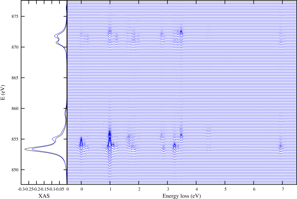
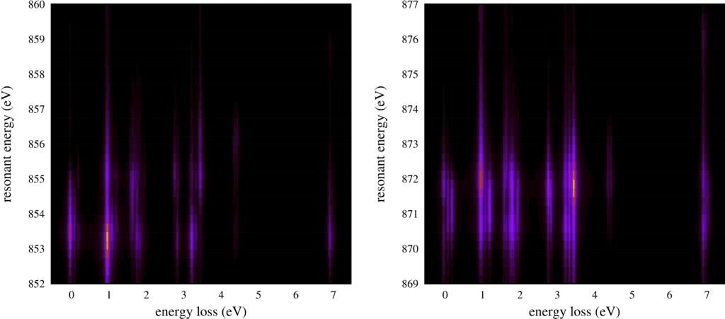
It produces two plots.

The first shows on the left the XAS spectra in black and the integrated RIXS spectra (FY) in blue. The resonant enhanced $d$-$d$ excitations are shown in the right plot.

The second plot shows the same RIXS spectra, but now as an intensity map.

The text output of the script is:

RIXS_L23M45.out

  #    <E>      <S^2>    <L^2>    <J^2>    <S_x^3d> <L_x^3d> <S_y^3d> <L_y^3d> <S_z^3d> <L_z^3d> <l.s>    <F[2]>   <F[4]>   <Neg^3d> <Nt2g^3d><Neg^Ld> <Nt2g^Ld><N^3d>
  1   -3.503    1.999   12.000   15.095   -0.370   -0.115   -0.370   -0.115   -0.741   -0.230   -0.305   -1.042   -0.924    2.186    5.990    3.825    6.000    8.175 
  2   -3.395    1.999   12.000   15.160   -0.002   -0.000   -0.002   -0.000   -0.003   -0.001   -0.322   -1.043   -0.925    2.189    5.988    3.823    6.000    8.178 
  3   -3.286    1.999   12.000   15.211    0.369    0.113    0.369    0.113    0.737    0.227   -0.336   -1.043   -0.925    2.193    5.987    3.820    6.000    8.180 
Start of LanczosTriDiagonalizeKrylovMC
Start of LanczosTriDiagonalizeKrylovMC
Finished calculating the spectra now start plotting.
This might take more time than the calculation