This is an old revision of the document!
XAS
Example three calculates the $2p$ to $3d$ x-ray absorption spectra of transition metal compounds in cubic symmetry. It does so on a crystal field theory level. (Not the most accurate, but very informative. Ligand field calculations can be found later in the tutorials) As input it requires the ion name, the scaling factor for the Slater integrals, the size of the crystal field, a possible magnetic field and a temperature. The output contains the x-ray absorption spectra for all possible polarizations. Besides plots of a few standard polarizations the conductivity tensor is given, which allows one to create any experimental geometry possible.
This is a nice little script to play with and learn what x-ray absorption spectroscopy measures. For example have a look how the linear and circular dichroism change in NiO (Ni$^{2+}$ with 10Dq=1.1, red=0.9 or so) as a function of temperature. You can see these in the conductivity tensor.
The configuration file is:
- conf.in
-- 3d ion (e.g. Sc ... Cu) :
ion = "Ni"
-- Universal scaling parameter for the Slater integrals (beta):
beta = 0.90
-- Cubic Crystal Field Strength (10Dq) [eV]
tenDq = 1.1
-- External magnetic field Bext [Tesla]
Bx = 5 ; By = 0 ; Bz = 10
-- Temperature [Kelvin]
T = 1
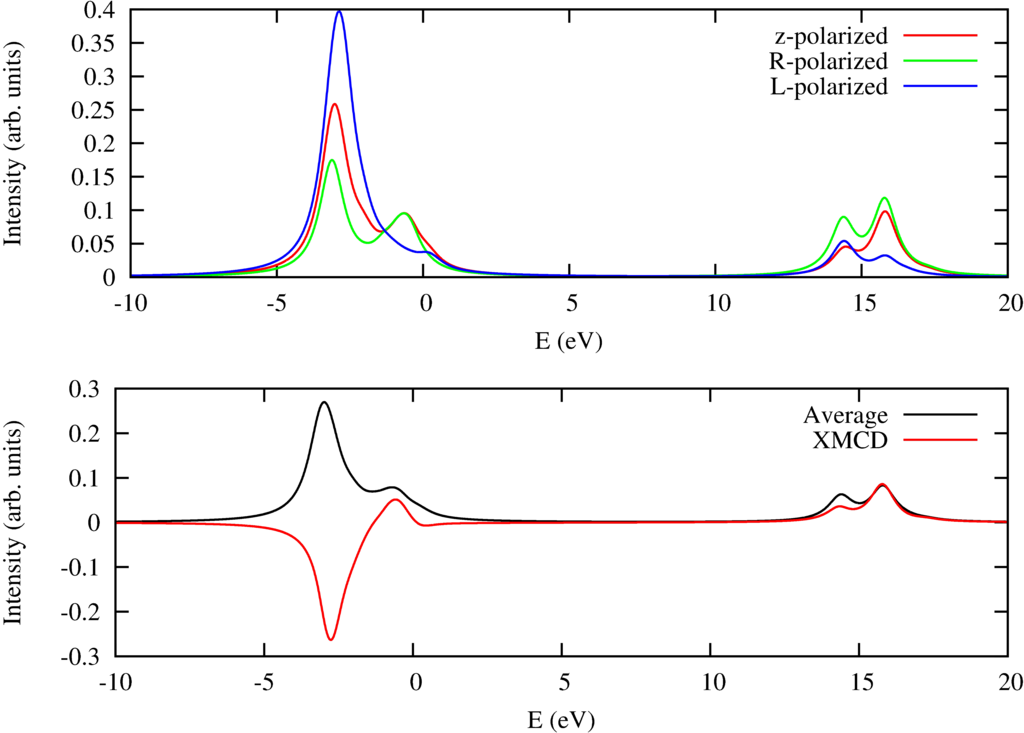
$L_{2,3}$ x-ray absorption spectra of Ni$^{2+}$ including magnetic circular dichroism.
Besides some text this program also creates plots of the x-ray absorption spectra. In the configuration file the magnetic field is set in the $(102)$ direction. The temperature is $1$ Kelvin and as the field size in the $z$ direction is 10 Tesla the Ni ion will be fully magnetically polarized. One can calculate the magnetic circular dichroic spectra by calculating the spectra for left and right circular polarized light and calculating the difference. This is done in this example and in the figure above one can see in the top pannel the XAS for $z$, $R$ (right circular) and $L$ (left circular) polarized light. The bottom pannel shows the isotropic spectra and the magnetic circular dichroic spectrum.
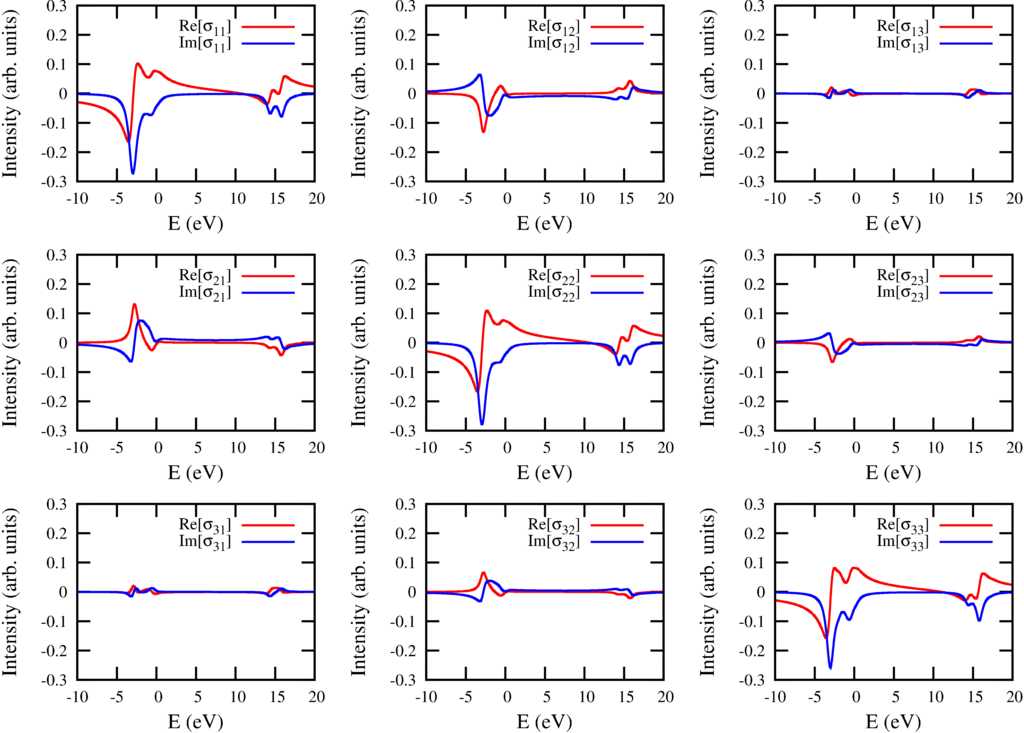
The conductivity tensor for excitations from $2p$ to $3d$ in Ni$^{2+}$
In principle one can calculate the spectra for any magnetic field direction, but also for any polarization direction. The Poyinting vector must not be in the $z$ direction and there are thus infinite possibilities to define left circular polarized light. In optics this is solved by calculating the optical conductivity tensor. This is a three by three matrix that describes the optical properties of the material for any posible polarization. If $\sigma(\omega)$ is the energy dependent conductivity tensor (three by three matrix) and $\varepsilon$ the polarization (a vector of length three) then the absorption is give as: $I_{XAS} = -\mathrm{Im}[\varepsilon^* \cdot \sigma(\omega) \cdot \varepsilon$]. The conductivity tensor for Ni$^{2+}$ with a field in the $(102)$ direction is shown in the figure above.
The figure above shows several interesting features. The diagonal elements show magnetic linear dichroism, but also some of the off diagonal elements are influenced by magnetic linear dichroism. The $yz$ component for example is symmetric (equal to the $zy$ component) and also given by a magnetic linear dichroic effect. (See Phys. Rev. B 82 094402 (2010)). The magnetic circular dichroism due to the field in the $z$ direction can be found as the antisymmetric part of $xy$ and $yx$. The magnetic circular dichroism due to the field in the $x$ direction can be found as the antisymmetric part of $yz$ and $zy$.
Information on the ground state is given in the text output, which is:
- XAS.out
--> This program is the spectra calculator.
--> Assuming a specific ionic configuration for Me^{2+} , the L-edge spectra are produced and plotted in a separate file.

--> Chosen parameters are as follows:
  Ion   beta       10Dq       Bext(x)      Bext(y)      Bext(z)       Temperature
  Ni    0.9000000  1.1000000  5.0000000  0.0000000   10.0000000       1.00

---> Setting up the Slater Integrals ...
---> Initial values are taken from M.W.Haverkort's PhD Thesis (p.156)


--> Assumed initial configuration: 2p6d8
--> INITIAL STATE PARAMETERS
  F0dd    F2dd    F4dd    zeta_3d
 0.5666 11.0097  6.8373  0.0830

--> Assumed final configuration: 2p5d9
--> FINAL STATE PARAMETERS
  F0dd    F2dd    F4dd    zeta_3d zeta_2p F2pd    G1pd    G3pd
 0.6025 11.7045  7.2756  0.1020 11.5070  6.9480  5.2047  2.9610

--> Calculating the lowest	45	eigenstates...

--> Ground state properties

  <E>    <S^2>  <L^2>  <J^2>  <S_z>  <L_z>  <l.s>  <F[2]> <F[4]> <Neg> <Nt2g>
-2.706  1.999 12.000 15.154 -0.889 -0.266 -0.334 -1.020 -0.878  2.011  5.989
-2.705  1.999 12.000 15.146 -0.000 -0.004 -0.332 -1.020 -0.878  2.011  5.989
-2.703  1.999 12.000 15.138  0.889  0.257 -0.330 -1.020 -0.878  2.011  5.989
-1.640  1.988 11.988 16.790 -0.167 -0.152 -0.873 -1.019 -0.877  3.008  4.992
-1.640  1.988 11.988 16.795 -0.012  0.001 -0.875 -1.019 -0.877  3.008  4.992
-1.621  1.999 12.000 15.825 -0.442 -0.029 -0.484 -1.020 -0.878  3.007  4.993
-1.621  1.999 12.000 15.835  0.157  0.103 -0.487 -1.020 -0.878  3.007  4.993
-1.620  1.999 12.000 15.840  0.441  0.078 -0.488 -1.020 -0.878  3.008  4.992
-1.570  1.997 11.989 12.550 -0.436 -0.134  0.265 -1.020 -0.877  2.996  5.004
-1.569  1.997 11.989 12.553 -0.058  0.005  0.265 -1.020 -0.877  2.996  5.004
-1.568  1.997 11.989 12.557  0.450  0.122  0.264 -1.020 -0.877  2.996  5.004
-1.549  2.000 12.000 12.001  0.068 -0.014  0.500 -1.020 -0.878  3.000  5.000
-0.944  1.995 11.483 18.926 -0.035 -0.036 -1.474 -1.003 -0.887  3.584  4.416
-0.876  1.999 11.421 15.293 -0.448  0.776 -0.506 -1.002 -0.887  3.568  4.432
-0.876  1.999 11.421 15.303  0.035  0.014 -0.509 -1.002 -0.887  3.569  4.431
-0.876  1.999 11.422 15.309  0.419 -0.769 -0.510 -1.002 -0.887  3.569  4.431
-0.797  1.726 10.766  9.049 -0.012  0.023 -0.081 -0.981 -0.878  3.334  4.666
-0.797  1.726 10.766  9.050  0.011  0.010 -0.081 -0.981 -0.878  3.334  4.666
-0.766  1.997 11.279  9.961 -0.427  0.434  0.788 -0.998 -0.890  3.544  4.456
-0.766  1.997 11.280  9.957  0.006  0.001  0.789 -0.998 -0.890  3.544  4.456
-0.766  1.997 11.280  9.952  0.450 -0.423  0.790 -0.998 -0.890  3.544  4.456
-0.489  0.290  9.837  9.162  0.000 -0.004  1.144 -0.902 -0.808  2.295  5.705
-0.489  0.290  9.837  9.162  0.000 -0.001  1.144 -0.902 -0.808  2.295  5.705
 0.459  0.151  7.374  7.664 -0.032 -0.490 -0.716 -0.887 -0.805  3.132  4.868
 0.460  0.150  7.379  7.668 -0.000  0.003 -0.715 -0.887 -0.805  3.132  4.868
 0.460  0.150  7.384  7.672  0.032  0.489 -0.714 -0.887 -0.805  3.132  4.868
 0.804  0.030 18.827 18.853 -0.000 -0.016  0.042 -0.767 -0.843  2.420  5.580
 0.923  1.992  2.783  6.359 -0.098 -0.081 -0.304 -0.737 -1.034  3.446  4.554
 0.923  1.992  2.782  6.358 -0.008  0.005 -0.306 -0.737 -1.034  3.446  4.554
 0.953  1.853  3.252  6.569 -0.417 -0.343  0.404 -0.749 -1.017  3.429  4.571
 0.953  1.853  3.250  6.569  0.085  0.078  0.402 -0.749 -1.017  3.429  4.571
 0.954  1.853  3.250  6.569  0.414  0.364  0.402 -0.749 -1.017  3.428  4.572
 0.987  1.994  2.636  2.910 -0.437 -0.386  0.409 -0.732 -1.037  3.421  4.579
 0.988  1.994  2.636  2.909 -0.020  0.017  0.409 -0.732 -1.037  3.420  4.580
 0.989  1.994  2.636  2.909  0.454  0.372  0.409 -0.732 -1.037  3.420  4.580
 1.019  1.972  2.755  1.287  0.028 -0.024  0.736 -0.731 -1.036  3.402  4.598
 1.264  0.009 19.943 19.958 -0.002 -0.448  0.084 -0.776 -0.855  3.003  4.997
 1.264  0.009 19.943 19.958  0.000  0.008  0.084 -0.776 -0.855  3.003  4.997
 1.265  0.009 19.943 19.958  0.002  0.444  0.085 -0.776 -0.855  3.003  4.997
 2.030  0.004 16.629 16.635 -0.000 -0.060  0.119 -0.810 -0.836  3.917  4.083
 2.030  0.004 16.628 16.635  0.000  0.010  0.119 -0.810 -0.836  3.917  4.083
 2.104  0.004 18.097 18.103  0.000 -1.807  0.090 -0.795 -0.845  3.888  4.112
 2.105  0.004 18.101 18.107  0.000  0.054  0.090 -0.795 -0.845  3.888  4.112
 2.106  0.004 18.106 18.112 -0.000  1.820  0.090 -0.795 -0.845  3.888  4.112
 5.913  0.003  0.936  0.933  0.000  0.000  0.196 -0.581 -0.585  3.594  4.406

Now the finite temperature properties will be calculated.
Boltzmann averaging of the M=2Ms+Ml operator and of the X-ray absorption spectra.

Partition function is sufficiently converged after Npsi=	2
Z,dZ	1.0000000364703	1.3291678830223e-15

For a magnetic field of ( 5.000000 0.000000 10.000000 ) Tesla
At temperature T=1.000000 Kelvin, the magnetic moment is:
     Spin      Orbital   Total
x    0.44461   0.13279   1.02202
y    0.00000   0.00000   0.00000
z    0.88920   0.26553   2.04393
Printing the components of the conductivity tensor (sigma[i,j])
Printing the XAS spectra
Prepare gnuplot-file for XAS spectra
Prepare gnuplot-file for Sigma

Execute the gnuplot to produce plots and convert the output into a pdf-file
FINISHED
For completeness, the actual code is:
- XAS.Quanty
-- script contributed by Yaroslav Kvashnin

-- Minimize the output of the program, i.e. for longer calculations
-- the program tells the user what it is doing. For these short
-- examples the result is instant.
Verbosity(0)

print("--> This program is the spectra calculator.")
print("--> Assuming a specific ionic configuration for Me^{2+} , the L-edge spectra are produced and plotted in a separate file.")
print("")
print("--> Chosen parameters are as follows:")

dofile("conf.in")

io.write("  Ion   beta       10Dq       Bext(x)      Bext(y)      Bext(z)       Temperature","\n")
io.write(string.format("  %s    %2.7f  %2.7f  %2.7f  %2.7f   %2.7f       %2.2f ",ion,beta,tenDq,Bx,By,Bz,T))
io.write("\n")

print("")
print("---> Setting up the Slater Integrals ...")
print("---> Initial values are taken from M.W.Haverkort's PhD Thesis (p.156)")
print("")

if ion=="Cu" then
Nelec=9
-- initial state parameters
zeta_3d=0.102; F2dd=12.854; F4dd=7.980
--  final  state parameters
zeta_2p=13.498; F2pd=8.177; G1pd=6.169; G3pd=3.510
--  final  state parameters
Xzeta_3d=0.124; XF2dd=13.611; XF4dd=8.457

elseif ion=="Ni" then
Nelec=8
zeta_3d=0.083; F2dd=12.233; F4dd=7.597
zeta_2p=11.507; F2pd=7.720; G1pd=5.783; G3pd=3.290
Xzeta_3d=0.102; XF2dd=13.005; XF4dd=8.084

elseif ion=="Co" then
Nelec=7
zeta_3d=0.066; F2dd=11.604; F4dd=7.209
zeta_2p=9.748; F2pd=7.259; G1pd=5.394; G3pd=3.068
Xzeta_3d=0.083; XF2dd=12.395; XF4dd=7.707

elseif ion=="Fe" then
Nelec=6
zeta_3d=0.052; F2dd=10.965; F4dd=6.815
zeta_2p=8.200; F2pd=6.792; G1pd=5.000; G3pd=2.843
Xzeta_3d=0.067; XF2dd=11.778; XF4dd=7.327

elseif ion=="Mn" then
Nelec=5
zeta_3d=0.040; F2dd=10.315 ; F4dd=6.413
zeta_2p=6.846; F2pd=6.320  ; G1pd=4.603; G3pd=2.617
Xzeta_3d=0.053; XF2dd=11.154 ; XF4dd=6.942

elseif ion=="Cr" then
Nelec=4
zeta_3d=0.030; F2dd=9.648; F4dd=6.001
zeta_2p=5.668; F2pd=5.840; G1pd=4.201; G3pd=2.387
Xzeta_3d=0.041; XF2dd=10.521; XF4dd=6.551

elseif ion=="V" then
Nelec=3
zeta_3d=0.022; F2dd=8.961; F4dd=5.576
zeta_2p=4.650; F2pd=5.351; G1pd=3.792; G3pd=2.154
Xzeta_3d=0.031; XF2dd=9.875; XF4dd=6.152

elseif ion=="Ti" then
Nelec=2
zeta_3d=0.016; F2dd=8.243; F4dd=5.132
zeta_2p=3.776; F2pd=4.849; G1pd=3.376; G3pd=1.917
Xzeta_3d=0.023; XF2dd=9.21; XF4dd=5.744

elseif ion=="Sc" then
Nelec=1
zeta_3d=0.010; F2dd=0; F4dd=0
zeta_2p=3.032; F2pd=4.332; G1pd=2.950; G3pd=1.674
Xzeta_3d=0.017; XF2dd=8.530; XF4dd=5.321

else
print("Could not recognize the ion name...")
os.exit()
end

-- scaling with beta factor
F2dd=beta*F2dd; F4dd=beta*F4dd
F2pd=beta*F2pd; G1pd=beta*G1pd; G3pd=beta*G3pd
XF2dd=beta*XF2dd; XF4dd=beta*XF4dd

-- number of possible many-body states in the initial configuration
Npsi = fact(10) / (fact(Nelec) * fact(10-Nelec))

-- Bringing everything to the same units (eV)
T = T * EnergyUnits.Kelvin.value
Bx = Bx * EnergyUnits.Tesla.value
By = By * EnergyUnits.Tesla.value
Bz = Bz * EnergyUnits.Tesla.value

-- 10 d-electrons + 6 p-electrons
NFermion=16
NBoson=0
-- p-shell [dn]
IndexDn_2p={0,2,4}
-- p-shell [up]
IndexUp_2p={1,3,5}
-- d-shell [dn]
IndexDn_3d={6,8,10,12,14}
-- d-shell [up]
IndexUp_3d={7,9,11,13,15}

-- define the operators
OppSx   =NewOperator("Sx"   ,NFermion, IndexUp_3d, IndexDn_3d)
OppSy   =NewOperator("Sy"   ,NFermion, IndexUp_3d, IndexDn_3d)
OppSz   =NewOperator("Sz"   ,NFermion, IndexUp_3d, IndexDn_3d)
OppSsqr =NewOperator("Ssqr" ,NFermion, IndexUp_3d, IndexDn_3d)
OppSplus=NewOperator("Splus",NFermion, IndexUp_3d, IndexDn_3d)
OppSmin =NewOperator("Smin" ,NFermion, IndexUp_3d, IndexDn_3d)

OppLx   =NewOperator("Lx"   ,NFermion, IndexUp_3d, IndexDn_3d)
OppLy   =NewOperator("Ly"   ,NFermion, IndexUp_3d, IndexDn_3d)
OppLz   =NewOperator("Lz"   ,NFermion, IndexUp_3d, IndexDn_3d)
OppLsqr =NewOperator("Lsqr" ,NFermion, IndexUp_3d, IndexDn_3d)
OppLplus=NewOperator("Lplus",NFermion, IndexUp_3d, IndexDn_3d)
OppLmin =NewOperator("Lmin" ,NFermion, IndexUp_3d, IndexDn_3d)

OppJx   =NewOperator("Jx"   ,NFermion, IndexUp_3d, IndexDn_3d)
OppJy   =NewOperator("Jy"   ,NFermion, IndexUp_3d, IndexDn_3d)
OppJz   =NewOperator("Jz"   ,NFermion, IndexUp_3d, IndexDn_3d)
OppJsqr =NewOperator("Jsqr" ,NFermion, IndexUp_3d, IndexDn_3d)
OppJplus=NewOperator("Jplus",NFermion, IndexUp_3d, IndexDn_3d)
OppJmin =NewOperator("Jmin" ,NFermion, IndexUp_3d, IndexDn_3d)

Oppldots=NewOperator("ldots",NFermion, IndexUp_3d, IndexDn_3d)

-- define the coulomb operator
-- we here define the part depending on F0 seperately from the part depending on F2
-- when summing we can put in the numerical values of the slater integrals

OppF0 =NewOperator("U", NFermion, IndexUp_3d, IndexDn_3d, {1,0,0})
OppF2 =NewOperator("U", NFermion, IndexUp_3d, IndexDn_3d, {0,1,0})
OppF4 =NewOperator("U", NFermion, IndexUp_3d, IndexDn_3d, {0,0,1})

-- Crystal field operator for the d-shell
Akm = PotentialExpandedOnClm("Oh", 2, {0.6,-0.4})
OpptenDq = NewOperator("CF", NFermion, IndexUp_3d, IndexDn_3d, Akm)
Akm = PotentialExpandedOnClm("Oh",2,{1,0});
OppNeg = NewOperator("CF", NFermion, IndexUp_3d, IndexDn_3d, Akm)
Akm = PotentialExpandedOnClm("Oh",2,{0,1});
OppNt2g = NewOperator("CF", NFermion, IndexUp_3d, IndexDn_3d, Akm)

-- Spin-orbit coupling in 2p-shell
Oppcldots= NewOperator("ldots", NFermion, IndexUp_2p, IndexDn_2p)
-- core hole potentials:
-- direct
OppUpdF0 = NewOperator("U", NFermion, IndexUp_2p, IndexDn_2p, IndexUp_3d, IndexDn_3d, {1,0}, {0,0})
OppUpdF2 = NewOperator("U", NFermion, IndexUp_2p, IndexDn_2p, IndexUp_3d, IndexDn_3d, {0,1}, {0,0})
-- exchange
OppUpdG1 = NewOperator("U", NFermion, IndexUp_2p, IndexDn_2p, IndexUp_3d, IndexDn_3d, {0,0}, {1,0})
OppUpdG3 = NewOperator("U", NFermion, IndexUp_2p, IndexDn_2p, IndexUp_3d, IndexDn_3d, {0,0}, {0,1})

t=math.sqrt(1/2);

-- setting up the transition operators with various polarisations
-- Dipole X
Akm = {{1,-1,t},{1, 1,-t}} ;
TXASx = NewOperator("CF", NFermion, IndexUp_3d, IndexDn_3d, IndexUp_2p, IndexDn_2p, Akm)
-- Dipole Y
Akm = {{1,-1,t*I},{1, 1,t*I}} ;
TXASy = NewOperator("CF", NFermion, IndexUp_3d, IndexDn_3d, IndexUp_2p, IndexDn_2p, Akm)
-- Dipole Z
Akm = {{1,0,1}} ;
TXASz = NewOperator("CF", NFermion, IndexUp_3d, IndexDn_3d, IndexUp_2p, IndexDn_2p, Akm)

TXASxpy  =  t*(TXASx + TXASy)
TXASypz  =  t*(TXASy + TXASz)
TXASzpx  =  t*(TXASz + TXASx)
TXASxpiy =  t*(TXASx + I * TXASy)
TXASypiz =  t*(TXASy + I * TXASz)
TXASzpix =  t*(TXASz + I * TXASx)

--- right circular polarisation
TXASr = t*(TXASx - I * TXASy)
---  left circular polarisation
TXASl =-t*(TXASx + I * TXASy)

------------------------------------------------
----- Input parameters for the Hamiltonian -----
-- in crystal field theory U drops out of the equation
U       =  0.000
F0dd    = U+(F2dd+F4dd)*2/63
XF0dd   = U+(XF2dd+XF4dd)*2/63
-- in crystal field theory U drops out of the equation
Upd     =  0.000
F0pd    =  Upd + G1pd*1/15 + G3pd*3/70

print("")
io.write(string.format("--> Assumed initial configuration: 2p6d%i", Nelec))
llist = {F0dd, F2dd, F4dd, zeta_3d}
print("")
print("--> INITIAL STATE PARAMETERS")
io.write("  F0dd    F2dd    F4dd    zeta_3d\n")
for i=1,4 do
io.write(string.format("%7.4f ",llist[i]))
end
print("")
print("")
io.write(string.format("--> Assumed final configuration: 2p5d%i",Nelec+1))
llist2 = {XF0dd, XF2dd, XF4dd, Xzeta_3d, zeta_2p, F2pd, G1pd, G3pd}
print("")
print("--> FINAL STATE PARAMETERS")
io.write("  F0dd    F2dd    F4dd    zeta_3d zeta_2p F2pd    G1pd    G3pd \n")
for i=1,8 do
io.write(string.format("%7.4f ",llist2[i]))
end
print("")

-- initial state Hamiltonian
Hamiltonian =  F0dd*OppF0 + F2dd*OppF2 + F4dd*OppF4 + tenDq*OpptenDq + zeta_3d*Oppldots
Hamiltonian = Hamiltonian + Bx * (2*OppSx + OppLx) + By * (2*OppSy + OppLy) + Bz * (2*OppSz + OppLz)

-- final state Hamiltonian
XASHamiltonian = XF0dd*OppF0 + XF2dd*OppF2 + XF4dd*OppF4 + tenDq*OpptenDq + Xzeta_3d*Oppldots + zeta_2p * Oppcldots + F2pd * OppUpdF2 + G1pd * OppUpdG1 + G3pd * OppUpdG3
XASHamiltonian = XASHamiltonian + Bx * (2*OppSx + OppLx) + By * (2*OppSy + OppLy) + Bz * (2*OppSz + OppLz)

-- in order to make sure we have a filling of 2 electrons we need to define some restrictions
StartRestrictions = {NFermion, NBoson, {"111111 0000000000",6,6}, {"000000 1111111111",Nelec,Nelec}}

print("")
print("--> Calculating the lowest", Npsi ,"eigenstates...")
psiList = Eigensystem(Hamiltonian, StartRestrictions, Npsi)


oppList={Hamiltonian, OppSsqr, OppLsqr, OppJsqr, OppSz, OppLz, Oppldots, OppF2, OppF4, OppNeg, OppNt2g};


print("")
print("--> Ground state properties")
print("")

-- Energy of the lowest multiplet. To be shifted to 0 to get a proper partition function

Egrd=psiList[1] * Hamiltonian * psiList[1]

print("  <E>    <S^2>  <L^2>  <J^2>  <S_z>  <L_z>  <l.s>  <F[2]> <F[4]> <Neg> <Nt2g>");
for key,value in pairs(psiList) do
  expvalue = value * oppList * value
  for k,v in pairs(expvalue) do
    io.write(string.format("%6.3f ",Complex.Re(v)))
  end
  io.write("\n")
end


print("")
print("Now the finite temperature properties will be calculated.")
print("Boltzmann averaging of the M=2Ms+Ml operator and of the X-ray absorption spectra.")
print("")

Z=0
Mx =0
MSx=0
MLx=0
My =0
MSy=0
MLy=0
Mz =0
MSz=0
MLz=0
Spectra_z=0
Spectra_r=0
Spectra_l=0

--- Conductivity tensor
Sigma_X=0
Sigma_Y=0
Sigma_Z=0
Sigma_X_p_Y=0
Sigma_Y_p_Z=0
Sigma_Z_p_X=0
Sigma_X_p_IY=0
Sigma_Y_p_IZ=0
Sigma_Z_p_IX=0

Z = 0 ;

 for j=1, Npsi do
  dZ = math.exp(-(psiList[j] * Hamiltonian * psiList[j] - Egrd)/T)
  if (dZ < 0.000000001) then
    print("Partition function is sufficiently converged after Npsi=",j-1)
	print("Z,dZ",Z,dZ)
	break
  end
  Z  = Z  + dZ
  Mx  = Mx  - psiList[j] * (2 * OppSx + OppLx) * psiList[j] * math.exp(-(psiList[j] * Hamiltonian * psiList[j] - Egrd)/T)
  MSx = MSx - psiList[j] * (OppSx)             * psiList[j] * math.exp(-(psiList[j] * Hamiltonian * psiList[j] - Egrd)/T)
  MLx = MLx - psiList[j] * (OppLx)             * psiList[j] * math.exp(-(psiList[j] * Hamiltonian * psiList[j] - Egrd)/T)
  My  = My  - psiList[j] * (2 * OppSy + OppLy) * psiList[j] * math.exp(-(psiList[j] * Hamiltonian * psiList[j] - Egrd)/T)
  MSy = MSy - psiList[j] * (OppSy)             * psiList[j] * math.exp(-(psiList[j] * Hamiltonian * psiList[j] - Egrd)/T)
  MLy = MLy - psiList[j] * (OppLy)             * psiList[j] * math.exp(-(psiList[j] * Hamiltonian * psiList[j] - Egrd)/T)
  Mz  = Mz  - psiList[j] * (2 * OppSz + OppLz) * psiList[j] * math.exp(-(psiList[j] * Hamiltonian * psiList[j] - Egrd)/T)
  MSz = MSz - psiList[j] * (OppSz)             * psiList[j] * math.exp(-(psiList[j] * Hamiltonian * psiList[j] - Egrd)/T)
  MLz = MLz - psiList[j] * (OppLz)             * psiList[j] * math.exp(-(psiList[j] * Hamiltonian * psiList[j] - Egrd)/T)
  Spectra_z = Spectra_z + CreateSpectra(XASHamiltonian, TXASz, psiList[j], {{"Emin",-10}, {"Emax",20}, {"NE",3500}, {"Gamma",1.0}}) * exp(-(psiList[j] * Hamiltonian * psiList[j] - Egrd)/T)
  Spectra_r = Spectra_r + CreateSpectra(XASHamiltonian, TXASr, psiList[j], {{"Emin",-10}, {"Emax",20}, {"NE",3500}, {"Gamma",1.0}}) * exp(-(psiList[j] * Hamiltonian * psiList[j] - Egrd)/T)
  Spectra_l = Spectra_l + CreateSpectra(XASHamiltonian, TXASl, psiList[j], {{"Emin",-10}, {"Emax",20}, {"NE",3500}, {"Gamma",1.0}}) * exp(-(psiList[j] * Hamiltonian * psiList[j] - Egrd)/T)
  Sigma_X = Sigma_X + CreateSpectra(XASHamiltonian, TXASx, psiList[j],{{"Emin",-10}, {"Emax",20}, {"NE",3500}, {"Gamma",1.0}}) * exp(-(psiList[j] * Hamiltonian * psiList[j] - Egrd)/T)
  Sigma_Y = Sigma_Y + CreateSpectra(XASHamiltonian, TXASy, psiList[j],{{"Emin",-10}, {"Emax",20}, {"NE",3500}, {"Gamma",1.0}}) * exp(-(psiList[j] * Hamiltonian * psiList[j] - Egrd)/T)
  Sigma_Z = Sigma_Z + CreateSpectra(XASHamiltonian, TXASz, psiList[j],{{"Emin",-10}, {"Emax",20}, {"NE",3500}, {"Gamma",1.0}}) * exp(-(psiList[j] * Hamiltonian * psiList[j] - Egrd)/T)
  Sigma_X_p_Y = Sigma_X_p_Y + CreateSpectra(XASHamiltonian, TXASxpy, psiList[j], {{"Emin",-10}, {"Emax",20}, {"NE",3500}, {"Gamma",1.0}}) * exp(-(psiList[j] * Hamiltonian * psiList[j] - Egrd)/T)
  Sigma_Y_p_Z = Sigma_Y_p_Z + CreateSpectra(XASHamiltonian, TXASypz, psiList[j], {{"Emin",-10}, {"Emax",20}, {"NE",3500}, {"Gamma",1.0}}) * exp(-(psiList[j] * Hamiltonian * psiList[j] - Egrd)/T)
  Sigma_Z_p_X = Sigma_Z_p_X + CreateSpectra(XASHamiltonian, TXASzpx, psiList[j], {{"Emin",-10}, {"Emax",20}, {"NE",3500}, {"Gamma",1.0}}) * exp(-(psiList[j] * Hamiltonian * psiList[j] - Egrd)/T)
  Sigma_X_p_IY = Sigma_X_p_IY + CreateSpectra(XASHamiltonian, TXASxpiy, psiList[j], {{"Emin",-10}, {"Emax",20}, {"NE",3500}, {"Gamma",1.0}}) * exp(-(psiList[j] * Hamiltonian * psiList[j] - Egrd)/T)
  Sigma_Y_p_IZ = Sigma_Y_p_IZ + CreateSpectra(XASHamiltonian, TXASypiz, psiList[j], {{"Emin",-10}, {"Emax",20}, {"NE",3500}, {"Gamma",1.0}}) * exp(-(psiList[j] * Hamiltonian * psiList[j] - Egrd)/T)
  Sigma_Z_p_IX = Sigma_Z_p_IX + CreateSpectra(XASHamiltonian, TXASzpix, psiList[j], {{"Emin",-10}, {"Emax",20}, {"NE",3500}, {"Gamma",1.0}}) * exp(-(psiList[j] * Hamiltonian * psiList[j] - Egrd)/T)
 end;
Mx  = Mx  / Z
MSx = MSx / Z
MLx = MLx / Z
My  = My  / Z
MSy = MSy / Z
MLy = MLy / Z
Mz  = Mz  / Z
MSz = MSz / Z
MLz = MLz / Z
Spectra_z = Spectra_z/Z
Spectra_r = Spectra_r/Z
Spectra_l = Spectra_l/Z
Sigma_X = Sigma_X/Z
Sigma_Y = Sigma_Y/Z
Sigma_Z = Sigma_Z/Z
Sigma_X_p_Y = Sigma_X_p_Y/Z
Sigma_Y_p_Z = Sigma_Y_p_Z/Z
Sigma_Z_p_X = Sigma_Z_p_X/Z
Sigma_X_p_IY = Sigma_X_p_IY/Z
Sigma_Y_p_IZ = Sigma_Y_p_IZ/Z
Sigma_Z_p_IX = Sigma_Z_p_IX/Z

print("")

io.write(string.format("For a magnetic field of ( %f %f %f ) Tesla\n", Bx/EnergyUnits.Tesla.value, By/EnergyUnits.Tesla.value, Bz/EnergyUnits.Tesla.value))
io.write(string.format("At temperature T=%f Kelvin, the magnetic moment is:\n", T/EnergyUnits.Kelvin.value))
print("     Spin      Orbital   Total")
io.write(string.format("x  %9.5f %9.5f %9.5f\n", Complex.Re(MSx),Complex.Re(MLx),Complex.Re(Mx)))
io.write(string.format("y  %9.5f %9.5f %9.5f\n", Complex.Re(MSy),Complex.Re(MLy),Complex.Re(My)))
io.write(string.format("z  %9.5f %9.5f %9.5f\n", Complex.Re(MSz),Complex.Re(MLz),Complex.Re(Mz)))

Spectra_ave  = (Spectra_z + Spectra_l + Spectra_r)/3
Spectra_XMCD = (Spectra_r - Spectra_l)

Sigma_11 = Sigma_X
Sigma_22 = Sigma_Y
Sigma_33 = Sigma_Z

Sigma_12 = Sigma_X_p_Y - I * Sigma_X_p_IY - 0.5 * (1 - I) * (Sigma_X + Sigma_Y)
Sigma_21 = Sigma_X_p_Y + I * Sigma_X_p_IY - 0.5 * (1 + I) * (Sigma_Y + Sigma_X)

Sigma_13 = Sigma_Z_p_X + I * Sigma_Z_p_IX - 0.5 * (1 + I) * (Sigma_X + Sigma_Z)
Sigma_31 = Sigma_Z_p_X - I * Sigma_Z_p_IX - 0.5 * (1 - I) * (Sigma_Z + Sigma_X)

Sigma_23 = Sigma_Y_p_Z - I * Sigma_Y_p_IZ - 0.5 * (1 - I) * (Sigma_Y + Sigma_Z)
Sigma_32 = Sigma_Y_p_Z + I * Sigma_Y_p_IZ - 0.5 * (1 + I) * (Sigma_Z + Sigma_Y)


print("Printing the components of the conductivity tensor (sigma[i,j])")
Sigma_11.Print({{"file","Sigma11.dat"}})
Sigma_22.Print({{"file","Sigma22.dat"}})
Sigma_33.Print({{"file","Sigma33.dat"}})
Sigma_12.Print({{"file","Sigma12.dat"}})
Sigma_21.Print({{"file","Sigma21.dat"}})
Sigma_13.Print({{"file","Sigma13.dat"}})
Sigma_31.Print({{"file","Sigma31.dat"}})
Sigma_23.Print({{"file","Sigma23.dat"}})
Sigma_32.Print({{"file","Sigma32.dat"}})

print("Printing the XAS spectra")
Spectra_z.Print({{"file","XASSpecZ.dat"}})
Spectra_r.Print({{"file","XASSpecR.dat"}})
Spectra_l.Print({{"file","XASSpecL.dat"}})
Spectra_ave.Print({{"file","XASSpecAVER.dat"}})
Spectra_XMCD.Print({{"file","XASSpecXMCD.dat"}})

--  prepare the gnuplot output for XAS
gnuplotInput = [[
set autoscale   # scale axes automatically
set xtic auto   # set xtics automatically
set ytic auto   # set ytics automatically

set style line  1 lt 1 lw 2 lc rgb "#FF0000"
set style line  2 lt 1 lw 2 lc rgb "#00FF00"
set style line  3 lt 1 lw 2 lc rgb "#0000FF"
set style line  4 lt 1 lw 2 lc rgb "#000000"

set xlabel "E (eV)" font "Times,12"
set ylabel "Intensity (arb. units)" font "Times,12"

set out 'XASSpec.ps'
set size 1.0, 1.0
set terminal postscript portrait enhanced color "Times" 12

set multiplot layout 4, 1
plot "XASSpecZ.dat"    using 1:(-$3) title 'z-polarized' with lines ls 1,\
     "XASSpecR.dat"    using 1:(-$3) title 'R-polarized' with lines ls 2,\
     "XASSpecL.dat"    using 1:(-$3) title 'L-polarized' with lines ls 3
plot "XASSpecAVER.dat" using 1:(-$3) title 'Average' with lines ls 4,\
     "XASSpecXMCD.dat" using 1:(-$3) title 'XMCD' with lines ls 1
unset multiplot

]]

print("Prepare gnuplot-file for XAS spectra")
-- write the gnuplot script to a file
file = io.open("XASSpec.gnuplot", "w")
file:write(gnuplotInput)
file:close()

-- prepare the gnuplot output for Sigma
gnuplotInput = [[
set autoscale   # scale axes automatically
set xtic auto   # set xtics automatically
set ytic auto   # set ytics automatically
set style line  1 lt 1 lw 2 lc 1
set style line  2 lt 1 lw 2 lc 3

set xlabel "E (eV)" font "Times,10"
set ylabel "Intensity (arb. units)" font "Times,10"

set yrange [-0.3:0.3]

set out 'SigmaTensor.ps'
set size 1.0, 1.0
set terminal postscript portrait enhanced color  "Times" 8

set multiplot layout 6, 3

plot "Sigma11.dat" u 1:2 title 'Re[{/Symbol s}_{11}]' with lines ls 1,\
     "Sigma11.dat" u 1:3 title 'Im[{/Symbol s}_{11}]' with lines ls 2
plot "Sigma12.dat" u 1:2 title 'Re[{/Symbol s}_{12}]' with lines ls 1,\
     "Sigma12.dat" u 1:3 title 'Im[{/Symbol s}_{12}]' with lines ls 2
plot "Sigma13.dat" u 1:2 title 'Re[{/Symbol s}_{13}]' with lines ls 1,\
     "Sigma13.dat" u 1:3 title 'Im[{/Symbol s}_{13}]' with lines ls 2
plot "Sigma21.dat" u 1:2 title 'Re[{/Symbol s}_{21}]' with lines ls 1,\
     "Sigma21.dat" u 1:3 title 'Im[{/Symbol s}_{21}]' with lines ls 2
plot "Sigma22.dat" u 1:2 title 'Re[{/Symbol s}_{22}]' with lines ls 1,\
     "Sigma22.dat" u 1:3 title 'Im[{/Symbol s}_{22}]' with lines ls 2
plot "Sigma23.dat" u 1:2 title 'Re[{/Symbol s}_{23}]' with lines ls 1,\
     "Sigma23.dat" u 1:3 title 'Im[{/Symbol s}_{23}]' with lines ls 2
plot "Sigma31.dat" u 1:2 title 'Re[{/Symbol s}_{31}]' with lines ls 1,\
     "Sigma31.dat" u 1:3 title 'Im[{/Symbol s}_{31}]' with lines ls 2
plot "Sigma32.dat" u 1:2 title 'Re[{/Symbol s}_{32}]' with lines ls 1,\
     "Sigma32.dat" u 1:3 title 'Im[{/Symbol s}_{32}]' with lines ls 2
plot "Sigma33.dat" u 1:2 title 'Re[{/Symbol s}_{33}]' with lines ls 1,\
     "Sigma33.dat" u 1:3 title 'Im[{/Symbol s}_{33}]' with lines ls 2

unset multiplot
]]

print("Prepare gnuplot-file for Sigma")

-- write the gnuplot script to a file
file = io.open("SigmaTensor.gnuplot", "w")
file:write(gnuplotInput)
file:close()

print("")
print("Execute the gnuplot to produce plots and convert the output into a pdf-file")

-- call gnuplot to execute the script
os.execute("gnuplot XASSpec.gnuplot ; ps2pdf XASSpec.ps ; ps2eps XASSpec.ps ; mv XASSpec.eps temp.eps ; eps2eps temp.eps XASSpec.eps ; rm temp.eps")
os.execute("gnuplot SigmaTensor.gnuplot ; ps2pdf SigmaTensor.ps ; ps2eps SigmaTensor.ps ;  mv SigmaTensor.eps temp.eps ; eps2eps temp.eps SigmaTensor.eps ; rm temp.eps")

print("FINISHED")