nIXS $M_{4,5}$ ($d$-$d$ excitations)
Inelastic x-ray scattering IXS (non-resonant) nIXS or x-ray Raman scattering allows one to measure non-dipolar allowed transitions. A powerful technique to look at even $d$-$d$ transitions with well defined selection rules \cite{Haverkort:2007bv, vanVeenendaal:2008kv, Hiraoka:2011cq}, but can also be used to determine orbital occupations of rare-earth ions that are fundamentally not possible to determine using dipolar spectroscopy \cite{Willers:2012bz}.
This tutorial compares calculated spectra to experiment. In order to make the plots you need to download the experimental data. You can download them in a zip file here nio_data.zip. Please unpack this file and make sure to have the folders NiO_Experiment and NiO_Radial in the same folder as you do the calculations. And as always, if used in a publication, please cite the original papers that published the data.
This example shows low energy $d$-$d$ transitions in NiO. The input is:
- nIXS_M45.Quanty
-- This example calculates the d-d excitations in NiO using non-resonant Inelastic X-ray
-- Scattering. This is one of the most beautiful spectroscopy techniques as the selection
-- rules are very "simple" and straight forward.

-- We use the A^2 term of the interaction to make transitions between states with photons
-- of much higher energy. These photons now cary non negligible momentum and one can make
-- transitions beyond the dipole limit.

-- Here we look at k=2 and k=4 transitions between the Ni 3d orbitals

-- we set the output to a minimum
Verbosity(0)

-- define the basis of one particle spin-orbitals
-- we only need the d orbitals in this case
NF=10
NB=0
IndexDn_3d={0,2,4,6,8}
IndexUp_3d={1,3,5,7,9}

-- define operators on this basis
OppSx   =NewOperator("Sx"   ,NF, IndexUp_3d, IndexDn_3d)
OppSy   =NewOperator("Sy"   ,NF, IndexUp_3d, IndexDn_3d)
OppSz   =NewOperator("Sz"   ,NF, IndexUp_3d, IndexDn_3d)
OppSsqr =NewOperator("Ssqr" ,NF, IndexUp_3d, IndexDn_3d)
OppSplus=NewOperator("Splus",NF, IndexUp_3d, IndexDn_3d)
OppSmin =NewOperator("Smin" ,NF, IndexUp_3d, IndexDn_3d)

OppLx   =NewOperator("Lx"   ,NF, IndexUp_3d, IndexDn_3d)
OppLy   =NewOperator("Ly"   ,NF, IndexUp_3d, IndexDn_3d)
OppLz   =NewOperator("Lz"   ,NF, IndexUp_3d, IndexDn_3d)
OppLsqr =NewOperator("Lsqr" ,NF, IndexUp_3d, IndexDn_3d)
OppLplus=NewOperator("Lplus",NF, IndexUp_3d, IndexDn_3d)
OppLmin =NewOperator("Lmin" ,NF, IndexUp_3d, IndexDn_3d)

OppJx   =NewOperator("Jx"   ,NF, IndexUp_3d, IndexDn_3d)
OppJy   =NewOperator("Jy"   ,NF, IndexUp_3d, IndexDn_3d)
OppJz   =NewOperator("Jz"   ,NF, IndexUp_3d, IndexDn_3d)
OppJsqr =NewOperator("Jsqr" ,NF, IndexUp_3d, IndexDn_3d)
OppJplus=NewOperator("Jplus",NF, IndexUp_3d, IndexDn_3d)
OppJmin =NewOperator("Jmin" ,NF, IndexUp_3d, IndexDn_3d)

Oppldots=NewOperator("ldots",NF, IndexUp_3d, IndexDn_3d)

-- define the coulomb operator
-- we here define the part depending on F0 seperately from the part depending on F2
-- when summing we can put in the numerical values of the slater integrals

OppF0 =NewOperator("U", NF, IndexUp_3d, IndexDn_3d, {1,0,0})
OppF2 =NewOperator("U", NF, IndexUp_3d, IndexDn_3d, {0,1,0})
OppF4 =NewOperator("U", NF, IndexUp_3d, IndexDn_3d, {0,0,1})

-- define the crystal-field operator

Akm = PotentialExpandedOnClm("Oh", 2, {0.6,-0.4})
OpptenDq = NewOperator("CF", NF, IndexUp_3d, IndexDn_3d, Akm)

-- define number operators counting the number of eg and t2g electrons

Akm = PotentialExpandedOnClm("Oh", 2, {1,0})
OppNeg = NewOperator("CF", NF, IndexUp_3d, IndexDn_3d, Akm)
Akm = PotentialExpandedOnClm("Oh", 2, {0,1})
OppNt2g = NewOperator("CF", NF, IndexUp_3d, IndexDn_3d, Akm)

-- set some parameters (see PRB 85, 165113 (2012) for more information)
beta    =  0.8
U       =  0.000
F2dd    = 11.142 * beta
F4dd    =  6.874 * beta
F0dd    = U+(F2dd+F4dd)*2/63
tenDq   = 1.100
zeta_3d = 0.081
Bz      = 0.000001

-- create a parameter dependent Hamiltonian
Hamiltonian =  F0dd*OppF0 + F2dd*OppF2 + F4dd*OppF4 + tenDq*OpptenDq + zeta_3d*Oppldots + Bz*(2*OppSz + OppLz)


-- We saw in the previous example that NiO has a ground-state doublet with occupation
-- t2g^6 eg^2 and S=1 (S^2=S(S+1)=2). The next state is 1.1 eV higher in energy and thus
-- unimportant for the ground-state upto temperatures of 10 000 Kelvin. We thus restrict
-- the calculation to the lowest 3 eigenstates.
Npsi=3
-- We need a filling of 8 electrons in the 3d shell
StartRestrictions = {NF, NB, {"1111111111",8,8}}

-- And calculate the lowest 3 eigenfunctions
psiList = Eigensystem(Hamiltonian, StartRestrictions, Npsi)

-- In order to get some information on these eigenstates it is good to plot expectation values
-- We first define a list of all the operators we would like to calculate the expectation value of
oppList={Hamiltonian, OppSsqr, OppLsqr, OppJsqr, OppSz, OppLz, Oppldots, OppF2, OppF4, OppNeg, OppNt2g};

-- next we loop over all operators and all states and print the expectation value
print(" <E>    <S^2>  <L^2>  <J^2>  <S_z>  <L_z>  <l.s>  <F[2]> <F[4]> <Neg>  <Nt2g>");
for i = 1,#psiList do
  for j = 1,#oppList do
    expectationvalue = Chop(psiList[i]*oppList[j]*psiList[i])
    io.write(string.format("%6.3f ",Complex.Re(expectationvalue)))
  end
  io.write("\n")
end

-- in order to calculate nIXS we need to determine the intensity ratio for the different multipole intensities
-- ( see PRL 99, 257401 (2007) for the formalism )
-- in short the A^2 interaction is expanded on spherical harmonics and Bessel functions
-- The 3d Wannier functions are expanded on spherical harmonics and a radial wave function
-- For the radial wave-function we calculate <R(r) | j_k(q r) | R(r)>
-- which defines the transition strength for the multipole of order k

-- The radial functions here are calculated for a Ni 2+ atom and stored in the folder NiO_Radial
-- more sophisticated methods can be used

-- read the radial wave functions
-- order of functions
-- r	1S	2S	2P	3S	3P	3D
file = io.open( "NiO_Radial/RnlNi_Atomic_Hartree_Fock", "r")
Rnl = {}
for line in file:lines() do
  RnlLine={}
  for i in string.gmatch(line, "%S+") do
    table.insert(RnlLine,i)
  end
  table.insert(Rnl,RnlLine)
end

-- some constants
a0      =  0.52917721092
Rydberg = 13.60569253
Hartree = 2*Rydberg

-- dd transitions from 3d (index 7 in Rnl) to 3d (index 7 in Rnl)
-- <R(r) | j_k(q r) | R(r)>
function RjRdd (q)
  Rj0R = 0
  Rj2R = 0
  Rj4R = 0
  dr = Rnl[3][1]-Rnl[2][1]
  r0 = Rnl[2][1]-2*dr
  for ir = 2, #Rnl, 1 do
    r = r0 + ir * dr
    Rj0R = Rj0R + Rnl[ir][7] * SphericalBesselJ(0,q*r) * Rnl[ir][7] * dr
    Rj2R = Rj2R + Rnl[ir][7] * SphericalBesselJ(2,q*r) * Rnl[ir][7] * dr
    Rj4R = Rj4R + Rnl[ir][7] * SphericalBesselJ(4,q*r) * Rnl[ir][7] * dr
  end
  return Rj0R, Rj2R, Rj4R
end

-- the angular part is given as C(theta_q, phi_q)^* C(theta_r, phi_r)
-- which is a potential expanded on spherical harmonics
function ExpandOnClm(k,theta,phi,scale)
  ret={}
  for m=-k, k, 1 do
    table.insert(ret,{k,m,scale * SphericalHarmonicC(k,m,theta,phi)})
  end
  return ret
end

-- define nIXS transition operators
function TnIXS_dd(q, theta, phi)
  Rj0R, Rj2R, Rj4R = RjRdd(q)
  k=0
  A0 = ExpandOnClm(k, theta, phi, I^k*(2*k+1)*Rj0R)
  T0 = NewOperator("CF", NF, IndexUp_3d, IndexDn_3d, A0)
  k=2
  A2 = ExpandOnClm(k, theta, phi, I^k*(2*k+1)*Rj2R)
  T2 = NewOperator("CF", NF, IndexUp_3d, IndexDn_3d, A2)
  k=4
  A4 = ExpandOnClm(k, theta, phi, I^k*(2*k+1)*Rj4R)
  T4 = NewOperator("CF", NF, IndexUp_3d, IndexDn_3d, A4)
  T = T0+T2+T4
  T.Chop()
  return T
end

-- q in units per a0 (if you want in units per A take 5*a0 to have a q of 5 per A)
q=4.5

print("for q=",q," per a0 (",q / a0," per A) The ratio of k=0, k=2 and k=4 transition strength is:",RjRdd(q))

-- define some transition operators
qtheta=0
qphi=0
Tq001 = TnIXS_dd(q,qtheta,qphi)

qtheta=Pi/2
qphi=Pi/4
Tq110 = TnIXS_dd(q,qtheta,qphi)

qtheta=acos(sqrt(1/3))
qphi=Pi/4
Tq111 = TnIXS_dd(q,qtheta,qphi)

qtheta=acos(sqrt(9/14))
qphi=acos(sqrt(1/5))
Tq123 = TnIXS_dd(q,qtheta,qphi)

-- calculate the spectra
nIXSSpectra = CreateSpectra(Hamiltonian, {Tq001, Tq110, Tq111, Tq123}, psiList, {{"Emin",-1}, {"Emax",6}, {"NE",3000}, {"Gamma",0.1}})

-- print the spectra to a file
nIXSSpectra.Print({{"file","NiOnIXS_dd.dat"}})

-- a gnuplot script to make the plots
gnuplotInput = [[
set autoscale
set xtic auto
set ytic auto
set style line  1 lt 1 lw 1 lc rgb "#FF0000"
set style line  2 lt 1 lw 1 lc rgb "#0000FF"
set style line  3 lt 1 lw 1 lc rgb "#00C000"
set style line  4 lt 1 lw 1 lc rgb "#800080"
set style line  5 lt 1 lw 3 lc rgb "#000000"

set xlabel "E (eV)" font "Times,12"
set ylabel "Intensity (arb. units)" font "Times,12"

set out 'NiOnIXS_dd.ps'
set size 1.0, 0.3
set terminal postscript portrait enhanced color  "Times" 12

set yrange [0:6.5]

plot "NiO_Experiment/NIXS_dd_JSR_16_469_2009" using 1:($2*0.01) title 'experiment' with filledcurves y1=0 ls 5 fs transparent solid 0.5,\
     "NiOnIXS_dd.dat" using 1:(-$15 -$17 -$19 +3.25) title 'q // 111' with lines ls  3,\
     "NiOnIXS_dd.dat" using 1:(-$21 -$23 -$25 +2.50) title 'q // 123' with lines ls  4,\
     "NiOnIXS_dd.dat" using 1:(-$9  -$11 -$13 +1.75) title 'q // 011' with lines ls  2,\
     "NiOnIXS_dd.dat" using 1:(-$3   -$5  -$7 +1.00) title 'q // 001' with lines ls  1
]]

-- write the gnuplot script to a file
file = io.open("NiOnIXS_dd.gnuplot", "w")
file:write(gnuplotInput)
file:close()

-- call gnuplot to execute the script
os.execute("gnuplot NiOnIXS_dd.gnuplot")
-- transform to pdf and eps
os.execute("ps2pdf NiOnIXS_dd.ps  ; ps2eps NiOnIXS_dd.ps  ;  mv NiOnIXS_dd.eps temp.eps  ; eps2eps temp.eps NiOnIXS_dd.eps  ; rm temp.eps")
The spectrum produced:
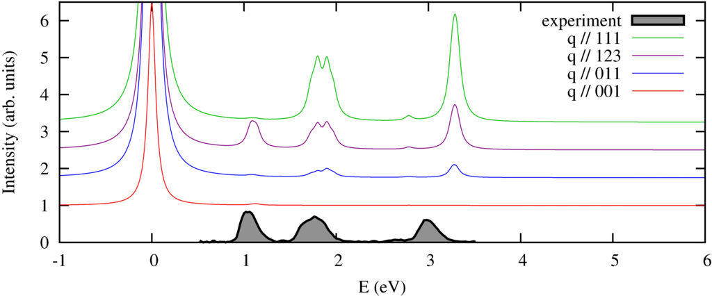
We calculate the spectrum in 4 different directions of momentum transfer. The experimental spectra (by Verbeni (2009) and Huotari (2008) et al.) are measured on a powder sample and thus do not show the strong momentum direction dependence. In previous measurements (Larson et al. (2007) and later in great detail by Hiroaka et al. (2009) this angular dependence has been observed, which agrees well with the theoretical predictions.
For completeness the output of the script is:
- nIXS_M45.out
 <E>    <S^2>  <L^2>  <J^2>  <S_z>  <L_z>  <l.s>  <F[2]> <F[4]> <Neg>  <Nt2g>
-2.444  1.999 12.000 15.118 -0.994 -0.285 -0.331 -1.020 -0.878  2.011  5.989
-2.444  1.999 12.000 15.118 -0.000 -0.000 -0.331 -1.020 -0.878  2.011  5.989
-2.444  1.999 12.000 15.118  0.994  0.285 -0.331 -1.020 -0.878  2.011  5.989
for q=	4.5	 per a0 (	8.5037675605428	 per A) The ratio of k=0, k=2 and k=4 transition strength is:	0.069703673179605	0.1609791731565	0.086144672158063