XAS $L_{2,3}$ as conductivity tensor
Absorption spectra are polarization dependent. In principle one can choose an infinite different number of polarizations. Calculating for each different experimental geometry (or polarization) a new spectrum is cumbersome and not needed. The material properties are given by the conductivity tensor. For dipole transitions a 3 by 3 matrix. The absorption spectra for a given experiment are then found by the relation: \begin{equation} I(\omega,\epsilon) = -\mathrm{Im}[\epsilon^* \cdot \sigma(\omega) \cdot \epsilon], \end{equation} with $\epsilon$ the polarization vector, $\omega$ the photon energy, $\sigma(\omega)$ the energy dependent conductivity tensor, and $I$ the measured intensity. Quanty can calculate the conductivity tensor. This is an extra option given to the function CreateSpectra (\{“Tensor”,true\}).
The example below calculates the conductivity tensor at the Ni $L_{2,3}$ edge. We show two different methods. The first calculates 9 spectra and by linear combining them retrieves the tensor. Method two uses a Block algorithm.
- XAS_tensor.Quanty
-- This tutorial calculates the 2p to 3d x-ray absorption spectra of Ni in NiO using
-- crystal field theory

-- the spectra are represented as a 3 by 3 tensor, the conductivity tensor. We show two
-- different methods to calculate this tensor, once creating 9 spectra with different
-- polarizations, once using the option Tensor in the CreateSpectra function

-- Within crystal-field theory the solid is approximated by a single atom in an effective
-- potential. Although an extremely crude approximation it is useful for some cases.
-- For correlated transition metal insulators it captures the right symmetry of the
-- localized open d-shell. It is useful to determine magnetic g-factors, energies of d-d
-- excitations or core level x-ray absorption. (2p to 3d excitations L23 edges)

-- One should notice that the effective crystal-field potential is an affective potential
-- it is there to mimic the interaction with neighboring ligand atoms. In real materials
-- there do not exist such large electro static potentials.

-- In order to do crystal-field theory for NiO we need to define a Ni d-shell.
-- A d-shell has 10 elements and we label again the even spin-orbitals to be spin down
-- and the odd spin-orbitals to be spin up. In order to calculate 2p to 3d excitations we
-- also need a Ni 2p shell. We thus have a total of 10+6=16 fermions, 6 Ni-2p and 10 Ni-3d
-- spin-orbitals

NF=16
NB=0
IndexDn_2p={0,2,4}
IndexUp_2p={1,3,5}
IndexDn_3d={6,8,10,12,14}
IndexUp_3d={7,9,11,13,15}

-- We define several operators acting on the Ni -3d shell

OppSx   =NewOperator("Sx"   ,NF, IndexUp_3d, IndexDn_3d)
OppSy   =NewOperator("Sy"   ,NF, IndexUp_3d, IndexDn_3d)
OppSz   =NewOperator("Sz"   ,NF, IndexUp_3d, IndexDn_3d)
OppSsqr =NewOperator("Ssqr" ,NF, IndexUp_3d, IndexDn_3d)
OppSplus=NewOperator("Splus",NF, IndexUp_3d, IndexDn_3d)
OppSmin =NewOperator("Smin" ,NF, IndexUp_3d, IndexDn_3d)

OppLx   =NewOperator("Lx"   ,NF, IndexUp_3d, IndexDn_3d)
OppLy   =NewOperator("Ly"   ,NF, IndexUp_3d, IndexDn_3d)
OppLz   =NewOperator("Lz"   ,NF, IndexUp_3d, IndexDn_3d)
OppLsqr =NewOperator("Lsqr" ,NF, IndexUp_3d, IndexDn_3d)
OppLplus=NewOperator("Lplus",NF, IndexUp_3d, IndexDn_3d)
OppLmin =NewOperator("Lmin" ,NF, IndexUp_3d, IndexDn_3d)

OppJx   =NewOperator("Jx"   ,NF, IndexUp_3d, IndexDn_3d)
OppJy   =NewOperator("Jy"   ,NF, IndexUp_3d, IndexDn_3d)
OppJz   =NewOperator("Jz"   ,NF, IndexUp_3d, IndexDn_3d)
OppJsqr =NewOperator("Jsqr" ,NF, IndexUp_3d, IndexDn_3d)
OppJplus=NewOperator("Jplus",NF, IndexUp_3d, IndexDn_3d)
OppJmin =NewOperator("Jmin" ,NF, IndexUp_3d, IndexDn_3d)

Oppldots=NewOperator("ldots",NF, IndexUp_3d, IndexDn_3d)

-- The Coulomb interaction

OppF0 =NewOperator("U", NF, IndexUp_3d, IndexDn_3d, {1,0,0})
OppF2 =NewOperator("U", NF, IndexUp_3d, IndexDn_3d, {0,1,0})
OppF4 =NewOperator("U", NF, IndexUp_3d, IndexDn_3d, {0,0,1})

-- The crystal-field operator

Akm = PotentialExpandedOnClm("Oh",2,{0.6,-0.4})
OpptenDq = NewOperator("CF", NF, IndexUp_3d, IndexDn_3d, Akm)

-- Count the number of eg and t2g electrons

Akm = PotentialExpandedOnClm("Oh",2,{1,0})
OppNeg = NewOperator("CF", NF, IndexUp_3d, IndexDn_3d, Akm)
Akm = PotentialExpandedOnClm("Oh",2,{0,1})
OppNt2g = NewOperator("CF", NF, IndexUp_3d, IndexDn_3d, Akm)

-- new for core level spectroscopy are operators that define the interaction acting on the
-- Ni-2p shell. There is actually only one of these interactions, which is the Ni-2p
-- spin-orbit interaction

Oppcldots= NewOperator("ldots", NF, IndexUp_2p, IndexDn_2p)

-- we also need to define the Coulomb interaction between the Ni 2p- and Ni 3d-shell
-- Again the interaction (e^2/(|r_i-r_j|)) is expanded on spherical harmonics. For the interaction
-- between two shells we need to consider two cases. For the direct interaction a 2p electron
-- scatters of a 3d electron into a 2p and 3d electron. The radial integrals involve
-- the square of a 2p radial wave function at coordinate 1 and the square of a 3d radial
-- wave function at coordinate 2. The transfer of angular momentum can either be 0 or 2.
-- These processes are called direct and the resulting Slater integrals are F[0] and F[2].
-- The second proces involves a 2p electron scattering of a 3d electron into the 3d shell
-- and at the same time the 3d electron scattering into a 2p shell. These exchange processes
-- involve radial integrals over the product of a 2p and 3d radial wave function. The transfer
-- of angular momentum in this case can be 1 or 3 and the Slater integrals are called G1 and G3.

-- In Quanty you can enter these processes by labeling 4 indices for the orbitals, once
-- the 2p shell with spin up, 2p shell with spin down, 3d shell with spin up and 3d shell with
-- spin down. Followed by the direct Slater integrals (F0 and F2) and the exchange Slater
-- integrals (G1 and G3)

-- Here we define the operators separately and later sum them with appropriate prefactors

OppUpdF0 = NewOperator("U", NF, IndexUp_2p, IndexDn_2p, IndexUp_3d, IndexDn_3d, {1,0}, {0,0})
OppUpdF2 = NewOperator("U", NF, IndexUp_2p, IndexDn_2p, IndexUp_3d, IndexDn_3d, {0,1}, {0,0})
OppUpdG1 = NewOperator("U", NF, IndexUp_2p, IndexDn_2p, IndexUp_3d, IndexDn_3d, {0,0}, {1,0})
OppUpdG3 = NewOperator("U", NF, IndexUp_2p, IndexDn_2p, IndexUp_3d, IndexDn_3d, {0,0}, {0,1})

-- next we define the dipole operator. The dipole operator is given as epsilon.r
-- with epsilon the polarization vector of the light and r the unit position vector
-- We can expand the position vector on (renormalized) spherical harmonics and use
-- the crystal-field operator to create the dipole operator.

-- x polarized light is defined as x = Cos[phi]Sin[theta] = sqrt(1/2) ( C_1^{(-1)} - C_1^{(1)})
Akm = {{1,-1,sqrt(1/2)},{1, 1,-sqrt(1/2)}}
TXASx = NewOperator("CF", NF, IndexUp_3d, IndexDn_3d, IndexUp_2p, IndexDn_2p, Akm)
-- y polarized light is defined as y = Sin[phi]Sin[theta] = sqrt(1/2) I ( C_1^{(-1)} + C_1^{(1)})
Akm = {{1,-1,sqrt(1/2)*I},{1, 1,sqrt(1/2)*I}}
TXASy = Chop(NewOperator("CF", NF, IndexUp_3d, IndexDn_3d, IndexUp_2p, IndexDn_2p, Akm))
-- z polarized light is defined as z = Cos[theta] = C_1^{(0)}
Akm = {{1,0,1}}
TXASz = NewOperator("CF", NF, IndexUp_3d, IndexDn_3d, IndexUp_2p, IndexDn_2p, Akm)


-- once all operators are defined we can set some parameter values.

-- the value of U drops out of a crystal-field calculation as the total number of electrons
-- is always the same
U       =  0.000
-- F2 and F4 are often referred to in the literature as J_{Hund}. They represent the energy
-- differences between different multiplets. Numerical values can be found in the back of
-- my PhD. thesis for example. http://arxiv.org/abs/cond-mat/0505214
F2dd    = 11.142
F4dd    =  6.874
-- F0 is not the same as U, although they are related. Unimportant in crystal-field theory
-- the difference between U and F0 is so important that I do include it here. (U=0 so F0 is not)
F0dd    = U+(F2dd+F4dd)*2/63
-- in crystal field theory U drops out of the equation, also true for the interaction between the
-- Ni 2p and Ni 3d electrons
Upd     =  0.000
-- The Slater integrals between the 2p and 3d shell, again the numerical values can be found
-- in the back of my PhD. thesis. (http://arxiv.org/abs/cond-mat/0505214)
F2pd    =  6.667
G1pd    =  4.922
G3pd    =  2.796
-- F0 is not the same as U, although they are related. Unimportant in crystal-field theory
-- the difference between U and F0 is so important that I do include it here. (U=0 so F0 is not)
F0pd    =  Upd + G1pd*1/15 + G3pd*3/70
-- tenDq in NiO is 1.1 eV as can be seen in optics or using IXS to measure d-d excitations
tenDq   =  1.100
-- the Ni 3d spin-orbit is small but finite
zeta_3d =  0.081
-- the Ni 2p spin-orbit is very large and should not be scaled as theory is quite accurate here
zeta_2p = 11.498
-- we can add a small magnetic field, just to get nice expectation values. (units in eV... )
Bz      = 0.000001
-- In mean field theory the neighboring Ni sites give an effective potential acting on the
-- spin only when magnetically ordered. This exchange field in NiO is 6 J with J=27 meV.
Hex     = 6*0.027 -- see Europhys. Lett., 32 259 (1995) [ and Phys. Rev. B 82, 094403 (2010) ]

-- the total Hamiltonian is the sum of the different operators multiplied with their prefactor
Hamiltonian = Chop(F0dd*OppF0 + F2dd*OppF2 + F4dd*OppF4 + tenDq*OpptenDq + zeta_3d*Oppldots + Bz*(2*OppSz+OppLz) + Hex*sqrt(1/6)*(OppSx+OppSy+2*OppSz))

-- We normally do not include core-valence interactions between filed and partially filled
-- shells as it drops out anyhow. For the XAS we thus need to define a "different"
-- (more complete) Hamiltonian.
XASHamiltonian = Hamiltonian + zeta_2p * Oppcldots + F0pd * OppUpdF0 + F2pd * OppUpdF2 + G1pd * OppUpdG1 + G3pd * OppUpdG3

-- We saw in the previous example that NiO has a ground-state doublet with occupation
-- t2g^6 eg^2 and S=1 (S^2=S(S+1)=2). The next state is 1.1 eV higher in energy and thus
-- unimportant for the ground-state upto temperatures of 10 000 Kelvin. We thus restrict
-- the calculation to the lowest 3 eigenstates.
Npsi=3
-- in order to make sure we have a filling of 8
-- electrons we need to define some restrictions
-- We need to restrict the occupation of the Ni-2p shell to 6 for the ground state and for
-- the Ni 3d-shell to 8.
StartRestrictions = {NF, NB, {"111111 0000000000",6,6}, {"000000 1111111111",8,8}}

-- And calculate the lowest 3 eigenfunctions
psiList = Eigensystem(Hamiltonian, StartRestrictions, Npsi)

-- In order to get some information on these eigenstates it is good to plot expectation values
-- We first define a list of all the operators we would like to calculate the expectation value of
oppList={Hamiltonian, OppSsqr, OppLsqr, OppJsqr, OppSx, OppLx, OppSy, OppLy, OppSz, OppLz, Oppldots, OppF2, OppF4, OppNeg, OppNt2g};

-- next we loop over all operators and all states and print the expectation value
print(" <E>    <S^2>  <L^2>  <J^2>  <S_x>  <L_x>  <S_y>  <L_y>  <S_z>  <L_z>  <l.s>  <F[2]> <F[4]> <Neg>  <Nt2g>");
for i = 1,#psiList do
  for j = 1,#oppList do
    expectationvalue = Chop(psiList[i]*oppList[j]*psiList[i])
    io.write(string.format("%6.3f ",Complex.Re(expectationvalue)))
  end
  io.write("\n")
end


-- calculating the spectra is simple and single line once all operators and wave-functions
-- are defined.

--------------------------- Method 1 -----------------------------
-- in order to create the tensor we define 9 spectra using operators that are combinations
-- of x, y and z polarized light

TXASypz  =  sqrt(1/2)*(TXASy + TXASz)
TXASzpx  =  sqrt(1/2)*(TXASz + TXASx)
TXASxpy  =  sqrt(1/2)*(TXASx + TXASy)
TXASypiz =  sqrt(1/2)*(TXASy + I * TXASz)
TXASzpix =  sqrt(1/2)*(TXASz + I * TXASx)
TXASxpiy =  sqrt(1/2)*(TXASx + I * TXASy)

TimeStart("Mehtod1")
XASSpectra = CreateSpectra(XASHamiltonian, {TXASx,TXASy,TXASz,TXASypz,TXASzpx,TXASxpy,TXASypiz,TXASzpix,TXASxpiy}, psiList[1], {{"Emin",-10}, {"Emax",20}, {"NE",3000}, {"Gamma",0.1}})
TimeEnd("Mehtod1")

-- Broaden these 9 spectra
TimeStart("Broaden")
XASSpectra.Broaden(0.4, {{-3.7, 0.45}, {-2.2, 0.65}, { 0.0, 0.65}, { 8  , 0.80}, {13.2, 0.80}, {14.0, 1.075}, {16.0, 1.075}})
TimeEnd("Broaden")

-- linear combine them into a tensor (note that the order here is given by the list of operators in the CreateSpectra function

XASSigma_method1 = Spectra.Sum(XASSpectra,{1,0,0,               0,0,0, 0, 0,0}, {-(1-I)/2,-(1-I)/2,0, 0,0,1, 0,0,-I}, {-(1+I)/2,0,-(1+I)/2, 0,1,0, 0,I,0 }
                                         ,{-(1+I)/2,-(1+I)/2,0, 0,0,1, 0, 0,I}, {0,1,0, 0,0,0, 0,0,0},                {0,-(1-I)/2,-(1-I)/2, 1,0,0, -I,0,0}
                                         ,{-(1-I)/2,0,-(1-I)/2, 0,1,0, 0,-I,0}, {0,-(1+I)/2,-(1+I)/2, 1,0,0, I,0, 0}, {0,0,1, 0,0,0, 0,0,0})

XASSigma_method1.Print({{"file","XASSigma_method1.dat"}})

-- prepare the gnuplot output for Sigma
gnuplotInput = [[
set autoscale   # scale axes automatically
set xtic auto   # set xtics automatically
set ytic auto   # set ytics automatically
set style line  1 lt 1 lw 2 lc 1
set style line  2 lt 1 lw 2 lc 3

set xlabel "E (eV)" font "Times,10"
set ylabel "Intensity (arb. units)" font "Times,10"

set yrange [-0.3:0.3]

set out 'SigmaTensor_method1.ps'
set size 1.0, 1.0
set terminal postscript portrait enhanced color  "Times" 8

set multiplot layout 6, 3

plot "XASSigma_method1.dat" u 1:2  title 'Re[{/Symbol s}_{xx}]' with lines ls 1,\
     "XASSigma_method1.dat" u 1:3  title 'Im[{/Symbol s}_{xx}]' with lines ls 2
plot "XASSigma_method1.dat" u 1:4  title 'Re[{/Symbol s}_{xy}]' with lines ls 1,\
     "XASSigma_method1.dat" u 1:5  title 'Im[{/Symbol s}_{xy}]' with lines ls 2
plot "XASSigma_method1.dat" u 1:6  title 'Re[{/Symbol s}_{xz}]' with lines ls 1,\
     "XASSigma_method1.dat" u 1:7  title 'Im[{/Symbol s}_{xz}]' with lines ls 2
plot "XASSigma_method1.dat" u 1:8  title 'Re[{/Symbol s}_{yx}]' with lines ls 1,\
     "XASSigma_method1.dat" u 1:9  title 'Im[{/Symbol s}_{yx}]' with lines ls 2
plot "XASSigma_method1.dat" u 1:10 title 'Re[{/Symbol s}_{yy}]' with lines ls 1,\
     "XASSigma_method1.dat" u 1:11 title 'Im[{/Symbol s}_{yy}]' with lines ls 2
plot "XASSigma_method1.dat" u 1:12 title 'Re[{/Symbol s}_{yz}]' with lines ls 1,\
     "XASSigma_method1.dat" u 1:13 title 'Im[{/Symbol s}_{yz}]' with lines ls 2
plot "XASSigma_method1.dat" u 1:14 title 'Re[{/Symbol s}_{zx}]' with lines ls 1,\
     "XASSigma_method1.dat" u 1:15 title 'Im[{/Symbol s}_{zx}]' with lines ls 2
plot "XASSigma_method1.dat" u 1:16 title 'Re[{/Symbol s}_{zy}]' with lines ls 1,\
     "XASSigma_method1.dat" u 1:17 title 'Im[{/Symbol s}_{zy}]' with lines ls 2
plot "XASSigma_method1.dat" u 1:18 title 'Re[{/Symbol s}_{zz}]' with lines ls 1,\
     "XASSigma_method1.dat" u 1:19 title 'Im[{/Symbol s}_{zz}]' with lines ls 2

unset multiplot
]]

print("Prepare gnuplot-file for Sigma")

-- write the gnuplot script to a file
file = io.open("SigmaTensor_method1.gnuplot", "w")
file:write(gnuplotInput)
file:close()

print("")
print("Execute the gnuplot to produce plots and convert the output into a pdf-file")

-- call gnuplot to execute the script
os.execute("gnuplot SigmaTensor_method1.gnuplot ; ps2pdf SigmaTensor_method1.ps ; ps2eps SigmaTensor_method1.ps ;  mv SigmaTensor_method1.eps temp.eps ; eps2eps temp.eps SigmaTensor_method1.eps ; rm temp.eps")

--------------------------- Method 2 -----------------------------


TimeStart("Mehtod2")
XASSigma_method2, SigmaTri = CreateSpectra(XASHamiltonian, {TXASx,TXASy,TXASz}, psiList[1], {{"Emin",-10}, {"Emax",20}, {"NE",3000}, {"Gamma",0.1}, {"Tensor",true}})
TimeEnd("Mehtod2")

-- Broaden these 9 spectra
TimeStart("Broaden")
XASSigma_method2.Broaden(0.4, {{-3.7, 0.45}, {-2.2, 0.65}, { 0.0, 0.65}, { 8  , 0.80}, {13.2, 0.80}, {14.0, 1.075}, {16.0, 1.075}})
TimeEnd("Broaden")

XASSigma_method2.Print({{"file","XASSigma_method2.dat"}})

-- prepare the gnuplot output for Sigma
gnuplotInput = [[
set autoscale   # scale axes automatically
set xtic auto   # set xtics automatically
set ytic auto   # set ytics automatically
set style line  1 lt 1 lw 2 lc 1
set style line  2 lt 1 lw 2 lc 3

set xlabel "E (eV)" font "Times,10"
set ylabel "Intensity (arb. units)" font "Times,10"

set yrange [-0.3:0.3]

set out 'SigmaTensor_method2.ps'
set size 1.0, 1.0
set terminal postscript portrait enhanced color  "Times" 8

set multiplot layout 6, 3

plot "XASSigma_method2.dat" u 1:2  title 'Re[{/Symbol s}_{xx}]' with lines ls 1,\
     "XASSigma_method2.dat" u 1:3  title 'Im[{/Symbol s}_{xx}]' with lines ls 2
plot "XASSigma_method2.dat" u 1:4  title 'Re[{/Symbol s}_{xy}]' with lines ls 1,\
     "XASSigma_method2.dat" u 1:5  title 'Im[{/Symbol s}_{xy}]' with lines ls 2
plot "XASSigma_method2.dat" u 1:6  title 'Re[{/Symbol s}_{xz}]' with lines ls 1,\
     "XASSigma_method2.dat" u 1:7  title 'Im[{/Symbol s}_{xz}]' with lines ls 2
plot "XASSigma_method2.dat" u 1:8  title 'Re[{/Symbol s}_{yx}]' with lines ls 1,\
     "XASSigma_method2.dat" u 1:9  title 'Im[{/Symbol s}_{yx}]' with lines ls 2
plot "XASSigma_method2.dat" u 1:10 title 'Re[{/Symbol s}_{yy}]' with lines ls 1,\
     "XASSigma_method2.dat" u 1:11 title 'Im[{/Symbol s}_{yy}]' with lines ls 2
plot "XASSigma_method2.dat" u 1:12 title 'Re[{/Symbol s}_{yz}]' with lines ls 1,\
     "XASSigma_method2.dat" u 1:13 title 'Im[{/Symbol s}_{yz}]' with lines ls 2
plot "XASSigma_method2.dat" u 1:14 title 'Re[{/Symbol s}_{zx}]' with lines ls 1,\
     "XASSigma_method2.dat" u 1:15 title 'Im[{/Symbol s}_{zx}]' with lines ls 2
plot "XASSigma_method2.dat" u 1:16 title 'Re[{/Symbol s}_{zy}]' with lines ls 1,\
     "XASSigma_method2.dat" u 1:17 title 'Im[{/Symbol s}_{zy}]' with lines ls 2
plot "XASSigma_method2.dat" u 1:18 title 'Re[{/Symbol s}_{zz}]' with lines ls 1,\
     "XASSigma_method2.dat" u 1:19 title 'Im[{/Symbol s}_{zz}]' with lines ls 2

unset multiplot
]]

print("Prepare gnuplot-file for Sigma")

-- write the gnuplot script to a file
file = io.open("SigmaTensor_method2.gnuplot", "w")
file:write(gnuplotInput)
file:close()

print("")
print("Execute the gnuplot to produce plots and convert the output into a pdf-file")

-- call gnuplot to execute the script
os.execute("gnuplot SigmaTensor_method2.gnuplot ; ps2pdf SigmaTensor_method2.ps ; ps2eps SigmaTensor_method2.ps ;  mv SigmaTensor_method2.eps temp.eps ; eps2eps temp.eps SigmaTensor_method2.eps ; rm temp.eps")

-------------------------- difference ------------------------

XASSigma_diff = XASSigma_method2 - XASSigma_method1


XASSigma_diff.Print({{"file","XASSigma_diff.dat"}})

-- prepare the gnuplot output for Sigma
gnuplotInput = [[
set autoscale   # scale axes automatically
set xtic auto   # set xtics automatically
set ytic auto   # set ytics automatically
set style line  1 lt 1 lw 2 lc 1
set style line  2 lt 1 lw 2 lc 3

set xlabel "E (eV)" font "Times,10"
set ylabel "Intensity (arb. units * 1000 000 000)" font "Times,10"

set yrange [-0.3:0.3]

scale = 1000000000

set out 'XASSigma_diff.ps'
set size 1.0, 1.0
set terminal postscript portrait enhanced color  "Times" 8

set multiplot layout 6, 3

plot "XASSigma_diff.dat" u 1:($2*scale)  title 'Re[{/Symbol s}_{xx}]' with lines ls 1,\
     "XASSigma_diff.dat" u 1:($3*scale)  title 'Im[{/Symbol s}_{xx}]' with lines ls 2
plot "XASSigma_diff.dat" u 1:($4*scale)  title 'Re[{/Symbol s}_{xy}]' with lines ls 1,\
     "XASSigma_diff.dat" u 1:($5*scale)  title 'Im[{/Symbol s}_{xy}]' with lines ls 2
plot "XASSigma_diff.dat" u 1:($6*scale)  title 'Re[{/Symbol s}_{xz}]' with lines ls 1,\
     "XASSigma_diff.dat" u 1:($7*scale)  title 'Im[{/Symbol s}_{xz}]' with lines ls 2
plot "XASSigma_diff.dat" u 1:($8*scale)  title 'Re[{/Symbol s}_{yx}]' with lines ls 1,\
     "XASSigma_diff.dat" u 1:($9*scale)  title 'Im[{/Symbol s}_{yx}]' with lines ls 2
plot "XASSigma_diff.dat" u 1:($10*scale) title 'Re[{/Symbol s}_{yy}]' with lines ls 1,\
     "XASSigma_diff.dat" u 1:($11*scale) title 'Im[{/Symbol s}_{yy}]' with lines ls 2
plot "XASSigma_diff.dat" u 1:($12*scale) title 'Re[{/Symbol s}_{yz}]' with lines ls 1,\
     "XASSigma_diff.dat" u 1:($13*scale) title 'Im[{/Symbol s}_{yz}]' with lines ls 2
plot "XASSigma_diff.dat" u 1:($14*scale) title 'Re[{/Symbol s}_{zx}]' with lines ls 1,\
     "XASSigma_diff.dat" u 1:($15*scale) title 'Im[{/Symbol s}_{zx}]' with lines ls 2
plot "XASSigma_diff.dat" u 1:($16*scale) title 'Re[{/Symbol s}_{zy}]' with lines ls 1,\
     "XASSigma_diff.dat" u 1:($17*scale) title 'Im[{/Symbol s}_{zy}]' with lines ls 2
plot "XASSigma_diff.dat" u 1:($18*scale) title 'Re[{/Symbol s}_{zz}]' with lines ls 1,\
     "XASSigma_diff.dat" u 1:($19*scale) title 'Im[{/Symbol s}_{zz}]' with lines ls 2

unset multiplot
]]

print("Prepare gnuplot-file for Sigma")

-- write the gnuplot script to a file
file = io.open("XASSigma_diff.gnuplot", "w")
file:write(gnuplotInput)
file:close()

print("")
print("Execute the gnuplot to produce plots and convert the output into a pdf-file")

-- call gnuplot to execute the script
os.execute("gnuplot XASSigma_diff.gnuplot ; ps2pdf XASSigma_diff.ps ; ps2eps XASSigma_diff.ps ;  mv XASSigma_diff.eps temp.eps ; eps2eps temp.eps XASSigma_diff.eps ; rm temp.eps")


---------------- overview of timing -------------------
TimePrint()
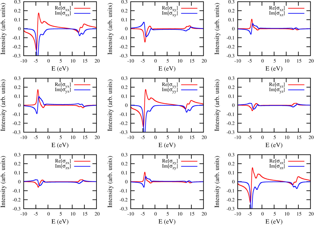
The resulting spectra are for method 1 are:
 |
| XAS spectra ($2p$ to $3d$) in form of a conductivity tensor ($\sigma$). For a particular polarization $\varepsilon$ the measured spectrum is $-\mathrm{Im}[\epsilon^* \cdot \sigma(\omega) \cdot \epsilon]$ |
|---|
The resulting spectra are for method 2 are:
 |
| XAS spectra ($2p$ to $3d$) in form of a conductivity tensor ($\sigma$). For a particular polarization $\varepsilon$ the measured spectrum is $-\mathrm{Im}[\epsilon^* \cdot \sigma(\omega) \cdot \epsilon]$ |
|---|
The difference is:
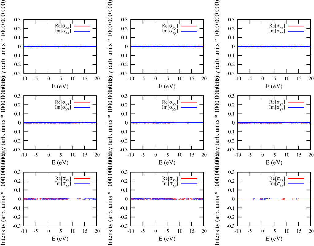 |
| Difference between calculation with method 1 and method 2 (should be zero) |
|---|
The output of the script is: <file Quanty_Output XAS_tensor.out> text produced as output Start of BlockGroundState. Converge 3 states to an energy with relative variance smaller than 1.490116119384766E-06
Start of BlockOperatorPsiSerialRestricted Outer loop 1, Number of Determinants: 45 45 last variance 2.335271462951932E+00 Start of BlockOperatorPsiSerialRestricted Start of BlockGroundState. Converge 3 states to an energy with relative variance smaller than 1.490116119384766E-06
Start of BlockOperatorPsiSerial <E> <S^2> <L^2> <J^2> <S_x> <L_x> <S_y> <L_y> <S_z> <L_z> <l.s> <F[2]> <F[4]> <Neg> <Nt2g> -2.882 1.999 12.000 15.052 -0.406 -0.117 -0.406 -0.117 -0.813 -0.234 -0.306 -1.020 -0.878 2.009 5.991 -2.721 1.999 12.000 15.142 -0.001 -0.000 -0.001 -0.000 -0.002 -0.001 -0.330 -1.020 -0.878 2.011 5.989 -2.560 1.999 12.000 15.211 0.405 0.116 0.405 0.116 0.810 0.233 -0.349 -1.020 -0.878 2.012 5.988 Start of LanczosTriDiagonalizeMC Start of LanczosTriDiagonalizeMC Start of LanczosTriDiagonalizeMC Start of LanczosTriDiagonalizeMC Start of LanczosTriDiagonalizeMC Start of LanczosTriDiagonalizeMC Start of LanczosTriDiagonalizeMC Start of LanczosTriDiagonalizeMC Start of LanczosTriDiagonalizeMC Spectra printed to file: XASSigma_method1.dat Prepare gnuplot-file for Sigma
Execute the gnuplot to produce plots and convert the output into a pdf-file Start of LanczosBlockTriDiagonalize Start of LanczosBlockTriDiagonalizeMC Spectra printed to file: XASSigma_method2.dat Prepare gnuplot-file for Sigma
Execute the gnuplot to produce plots and convert the output into a pdf-file Spectra printed to file: XASSigma_diff.dat Prepare gnuplot-file for Sigma
Execute the gnuplot to produce plots and convert the output into a pdf-file Timing results
 Total_time | NumberOfRuns | Running | Name
    0:00:04 |            1 |       0 | Mehtod1
    0:00:16 |            2 |       0 | Broaden
    0:00:01 |            1 |       0 | Mehtod2
###
===== Table of contents =====