Coulomb repulsion operator (U)

The Coulomb interaction is given as: $$\begin{equation} H = \sum_{i\neq j} \frac{1}{2} \frac{e^2}{|r_i-r_j|}, \end{equation}$$ whereby the sum runs over all electrons and the factor $1/2$ takes care of the double counting as each pair of electrons only repels once. In second quantization this Hamiltonian can be written as: $$\begin{equation} H = \sum_{\tau_1\tau_2\tau_3\tau_4} U_{\tau_1\tau_2\tau_3\tau_4} a^{\dagger}_{\tau_1}a^{\dagger}_{\tau_2}a^{\phantom{\dagger}}_{\tau_3}a^{\phantom{\dagger}}_{\tau_4}, \end{equation}$$ whereby $\tau$ labels the spin and orbital degrees of freedom.

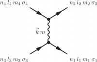
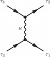Using Feynman diagrams this interaction can be depicted as two electrons entering with quantum numbers $\tau_4$ and $\tau_3$, exchanging an entity $\kappa$ and leaving with quantum numbers $\tau_1$ and $\tau_2$.

Calculating the Coulomb interaction is more difficult as one might expect. The interaction strength diverges when $r_1 = r_2$ and one needs to calculate the principle integral in three dimensions. A good way to evaluate this integral is to expand $1/|r_1-r_2|$ in spherical harmonics and separate the integrals over the angle for the integral over $r$. The angular integrals turn trivial with analytical solutions whereas the radial integral becomes non-divergent. If we assume spherical symmetry for the basis functions the result for the radial integrals are the Slater integrals. If the basis functions are more complex we still can expand these in spherical symmetry and the result is a sum over Slater integrals. The standard operator in Quanty implements the spherical case, the more general case can be created by importing results from DFT and will be discussed in those sections.

The expansion of $e^2/|r_1-r_2|$ is: $$\begin{equation} \sum_{i\neq j} \frac{1}{2} \frac{e^2}{|r_i-r_j|} = \sum_{i\neq j} \frac{1}{2}\sum_{k=0}^{\infty} \sum_{m=-k}^{m=k} \frac{4 \pi}{2k+1} \frac{\mathrm{Min}[r_i,r_j]^k}{\mathrm{Max}[r_i,r_j]^{k+1}} Y_m^{(k)}(\theta_i,\phi_i)Y_m^{(k)}(\theta_j,\phi_j)^*. \end{equation}$$

Expanding our basis states in spherical harmonics times radial wave functions the quantum number $\tau_i$ labels the set of quantum numbers $n_i,l_i,m_i,\sigma_i$. This allows us to separate the radial from angular part of the equation. Using that: $$\begin{eqnarray} &&\sum_i \sqrt{\frac{4 \pi}{2k+1}} Y_m^{(k)}(\theta_i,\phi_i) = \sum_i C_m^{(k)}(\theta_i,\phi_i) \\ \nonumber &&= \sum_{\tau_1,\tau_3} \delta_{\sigma_1,\sigma_3}\delta_{m,m_1-m_3} \left\langle Y_{m_1}^{(l_1)}(\theta,\phi) \left | C_m^{(k)}(\theta,\phi) \right | Y_{m_3}^{(l_3)}(\theta,\phi) \right\rangle a^{\dagger}_{\tau_1}a^{\phantom{\dagger}}_{\tau_3}, \end{eqnarray}$$ we can rewrite: $$\begin{equation} \sum_{i\neq j} \frac{1}{2}\sum_{k=0}^{\infty} \sum_{m=-k}^{m=k} \frac{4 \pi}{2k+1} Y_m^{(k)}(\theta_i,\phi_i)Y_m^{(k)}(\theta_j,\phi_j)^* \end{equation}$$ as: $$\begin{eqnarray} && \frac{1}{2}\sum_{k=0}^{k=\infty}\sum_{\tau_1,\tau_2,\tau_3,\tau_4} \delta_{\sigma_1,\sigma_3}\delta_{\sigma_2,\sigma_4}\delta_{m_4-m_2,m_1-m_3} \times \\ \nonumber && \left\langle Y_{m_1}^{(l_1)} \left | C_{m_1-m_3}^{(k)} \right | Y_{m_3}^{(l_3)} \right\rangle \left\langle Y_{m_4}^{(l_4)} \left | C_{m_4-m_2}^{(k)} \right | Y_{m_2}^{(l_2)} \right\rangle a^{\dagger}_{\tau_1}a^{\phantom{\dagger}}_{\tau_3} a^{\dagger}_{\tau_2}a^{\phantom{\dagger}}_{\tau_4}, \end{eqnarray}$$ which after reordering to normal order becomes: $$\begin{eqnarray} && -\frac{1}{2}\sum_{k=0}^{k=\infty}\sum_{\tau_1,\tau_2,\tau_3,\tau_4} \delta_{\sigma_1,\sigma_3}\delta_{\sigma_2,\sigma_4}\delta_{m_4-m_2,m_1-m_3} \times \\ \nonumber && \left\langle Y_{m_1}^{(l_1)} \left | C_{m_1-m_3}^{(k)} \right | Y_{m_3}^{(l_3)} \right\rangle \left\langle Y_{m_4}^{(l_4)} \left | C_{m_4-m_2}^{(k)} \right | Y_{m_2}^{(l_2)} \right\rangle a^{\dagger}_{\tau_1}a^{\dagger}_{\tau_2}a^{\phantom{\dagger}}_{\tau_3} a^{\phantom{\dagger}}_{\tau_4}. \end{eqnarray}$$

The radial part of the operator ($\frac{\mathrm{Min}[r_i,r_j]^k}{\mathrm{Max}[r_i,r_j]^{k+1}}$) is more difficult and will be cast into parameters: $$\begin{equation} R^{(k)}[\tau_1\tau_2\tau_3\tau_4]=e^2\int_0^{\infty}\int_0^{\infty}\frac{\mathrm{Min}[r_i,r_j]^k}{\mathrm{Max}[r_i,r_j]^{k+1}}R_1[r_i]R_2[r_j]R_3[r_i]R_4[r_j]r_i^2 r_j^2\mathrm{d}r_i\mathrm{d}r_j. \end{equation}$$

Which gives the final result: $$\begin{eqnarray} H &=& \sum_{\tau_1\tau_2\tau_3\tau_4} U_{\tau_1\tau_2\tau_3\tau_4} a^{\dagger}_{\tau_1}a^{\dagger}_{\tau_2}a^{\phantom{\dagger}}_{\tau_3}a^{\phantom{\dagger}}_{\tau_4},\\ \nonumber U_{\tau_1\tau_2\tau_3\tau_4} &=& -\frac{1}{2}\delta_{\sigma_1,\sigma_3}\delta_{\sigma_2,\sigma_4} \sum_{k=0}^{\infty}c^{(k)}[l_1,m_1;l_3,m_3]c^{(k)}[l_4,m_4;l_2,m_2]\\ \nonumber &&\quad \times R^{(k)}[\tau_1\tau_2\tau_3\tau_4],\\ \nonumber c^{(k)}[l_1,m_1;l_2,m_2] &=& \left\langle Y_{m_1}^{(l_1)} \left | C_{m_1-m_2}^{(k)} \right | Y_{m_2}^{(l_2)} \right\rangle. \end{eqnarray}$$

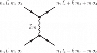Using angular momentum as a basis the scattering event described is given by the diagram on the left. An angular momentum $\vec{k}$ with a projection $m$ on the $z$ direction is exchanged.

Using conservation of angular momentum we can see that $|l_1-l_3| \leq k \leq |l_1+l_3|$ and $|l_2-l_4| \leq k \leq |l_2+l_4|$. This can be used to restrict the number of radial integrals one needs to compute.

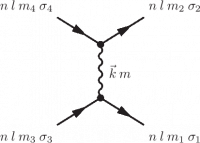For the case where $n_1=n_2=n_3=n_4$ and $l_1=l_2=l_3=l_4$, i.e. Coulomb repulsion within one shell one defines: $$\begin{equation} F^{(k)} = R^{(k)}[\tau_1\tau_2\tau_3\tau_4]. \end{equation}$$ In Quanty one can add this Coulomb operator as:

Example.Quanty

NewOperator("U", NF, IndexUp, IndexDn, SlaterIntegrals)

whereby SlaterIntegrals represents a list of $F^{(k)}$ with $k$ running from $0$ to $2l$ in steps of $2$, i.e. $k$ is even.

For a $d$ shell one can define:

Example.Quanty

OppF0 = NewOperator("U", NF, IndexUp, IndexDn, {1,0,0})
OppF2 = NewOperator("U", NF, IndexUp, IndexDn, {0,1,0})
OppF4 = NewOperator("U", NF, IndexUp, IndexDn, {0,0,1})

to get the Coulomb operator proportional to $F^{(0)}$, $F^{(2)}$ and $F^{(4)}$.

The Coulomb repulsion between two shells which does not change the number of electrons is given by a direct term ($n_1l_1=n_3l_3$ and $n_2l_2=n_4l_4$) and an indirect or exchange term ($n_1l_1=n_4l_4$ and $n_2l_2=n_3l_3$). We here assume that $n_1l_1\neq n_2l_2$. The direct term is given by the Slater integrals: $$\begin{equation} F^{(k)}=e^2\int_0^{\infty}\int_0^{\infty}\frac{\mathrm{Min}[r_i,r_j]^k}{\mathrm{Max}[r_i,r_j]^{k+1}}R_1[r_i]^2R_2[r_j]^2\mathrm{d}r_i\mathrm{d}r_j, \end{equation}$$ with $0 \leq k \leq \mathrm{Min}[2l_1,2l_2]$ in steps of 2, i.e. $k$ is even.

The indirect term is given by the exchange integrals: $$\begin{equation} G^{(k)}=e^2\int_0^{\infty}\int_0^{\infty}\frac{\mathrm{Min}[r_i,r_j]^k}{\mathrm{Max}[r_i,r_j]^{k+1}}R_1[r_i]R_1[r_j]R_2[r_i]R_2[r_j]\mathrm{d}r_i\mathrm{d}r_j, \end{equation}$$ with $|l_1-l_2| \leq k \leq |l_1+l_2|$ in steps of 2, i.e. $k$ is even if both $l_1$ and $l_2$ are even or odd and $k$ is odd if one of the angular momenta involved is even and the other is odd.

In Quanty one can implement these operators as:

Example.Quanty

NewOperator("U", NF, IndexUp_1, IndexDn_1, IndexUp_2, IndexDn_2, Fk, Gk)

For $l_1=1$ and $l_2=2$ one could define:

Example.Quanty

OppF0pd = NewOperator("U", NF, IndexUp_1, IndexDn_1, IndexUp_2, IndexDn_2, {1,0}, {0,0})
OppF2pd = NewOperator("U", NF, IndexUp_1, IndexDn_1, IndexUp_2, IndexDn_2, {0,1}, {0,0})
 
OppG1pd = NewOperator("U", NF, IndexUp_1, IndexDn_1, IndexUp_2, IndexDn_2, {0,0}, {1,0})
OppG3pd = NewOperator("U", NF, IndexUp_1, IndexDn_1, IndexUp_2, IndexDn_2, {0,0}, {0,1})

The Coulomb repulsion in the general case allows four different principle quantum numbers and angular momenta. The radial integral is given as: $$\begin{equation} R^{(k)}[n_1l_1\:n_2l_2\:n_3l_3\:n_4l_4]=e^2\int_0^{\infty}\int_0^{\infty}\frac{\mathrm{Min}[r_i,r_j]^k}{\mathrm{Max}[r_i,r_j]^{k+1}}R_{n_1l_1}[r_i]R_{n_2l_2}[r_j]R_{n_3l_3}[r_i]R_{n_4l_4}[r_j]\mathrm{d}r_i\mathrm{d}r_j, \end{equation}$$ with $\mathrm{Max}[|l_1-l_3|,|l_2-l_4|] \leq k \leq \mathrm{Min}[l_1+l_3,l_2+l_4]$ and $(l_1+l_3)$, $(l2_+l_4)$ either both even or both odd.

In Quanty one can implement these operators as:

Example.Quanty

NewOperator("U", NF, IndexUp_1, IndexDn_1, IndexUp_2, IndexDn_2, IndexUp_3, IndexDn_3, IndexUp_4, IndexDn_4, Rk)

For $l_1=3$, $l_2=0$, $l_3=2$ and $l_4=1$ one has $k=1$ and one could define:

Example.Quanty

OppR1pd = NewOperator("U", NF, IndexUp_1, IndexDn_1, IndexUp_2, IndexDn_2, IndexUp_3, IndexDn_3, IndexUp_4, IndexDn_4, {1})

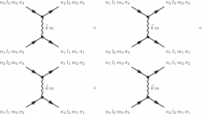
Note that in the general case you need to sum over all possible permutations of $n_1l_1$, $n_2l_2$, $n_3l_3$ and $n_4l_4$. Permuting $n_1l_1$ with $n_2l_2$ and at the same time $n_3l_3$ with $n_4l_4$ will not change the value and form of the operator. If $n_1l_1$ is different from $n_2l_2$ and $n_3l_3$ is different from $n_4l_4$ one can add a factor of two in front of the operator and only add one of the permutations. If one of the $n_1l_1$ is the same as $n_2l_2$ or $n_3l_3$ is the same as $n_4l_4$ a permutation will not lead to a new configuration and the factor of two disappears. If you just sum over all possible $n_il_i$ combinations things go right automatically.