This is an old revision of the document!
XAS $L_{2,3}$ partial excitations
In order to understand where a particular peak originates from one can look at the character of the excited state. Quanty works with Green's functions and we can not just look at the excited eigen-states as these are not really calculated. We can however modify the transition operator in order to understand where the spectra come from. The example below looks at excitations into the $t_{2g}$ and $e_g$ irreducible representations of the $d$ orbitals separately and looks at excitations from the $j=1/2$ and $j=3/2$ sub-shells of the $2p$ orbitals separately.
The input file is:
- XAS_partial.Quanty
-- In order to understand the different peaks in an absorption experiment one can look
-- at the character of the states one excites into.

-- Here we show the example of XAS making excitations from 2p to 3d.

-- Quanty works with Green's functions and we thus do not have final states from which we can
-- determine the character. We can however modify the transition operator such that it only excites
-- into, for example only t2g, or only eg electrons. Or we we can modify the transition operator
-- such that it only takes electrons from the 2p-j=1/2 or 2p-j=3/2 states. In the former one would
-- see which peaks arrise from the eg or t2g orbitals, in the later one would see the L2 and L3
-- edge separately in the case where j2p is a good quantum number. In the case where coulomb
-- repulsion mixes j2p=1/2 and j2p=3/2 states one sees this mixing.

-- In order to define the restricted transition operators we first rotate the orbital
-- basis of the operator to the orbital basis on which we want to select a subset of
-- orbitals. If we modify the rotation matrix to only keep a subset of the eigen-orbitals
-- we have the modification we want. Next we rotate the transition operator back to the
-- original basis we use throughout the calculation (l lz s sz) for the orbitals and ready
-- we are.

-- We copy tutorial 21 for the most part

-- In order to do crystal-field theory for NiO we need to define a Ni d-shell.
-- A d-shell has 10 elements and we label again the even spin-orbitals to be spin down
-- and the odd spin-orbitals to be spin up. In order to calculate 2p to 3d excitations we
-- also need a Ni 2p shell. We thus have a total of 10+6=16 fermions, 6 Ni-2p and 10 Ni-3d
-- spin-orbitals
NF=16
NB=0
IndexDn_2p={0,2,4}
IndexUp_2p={1,3,5}
IndexDn_3d={6,8,10,12,14}
IndexUp_3d={7,9,11,13,15}

-- just like in the previous example we define several operators acting on the Ni -3d shell

OppSx   =NewOperator("Sx"   ,NF, IndexUp_3d, IndexDn_3d)
OppSy   =NewOperator("Sy"   ,NF, IndexUp_3d, IndexDn_3d)
OppSz   =NewOperator("Sz"   ,NF, IndexUp_3d, IndexDn_3d)
OppSsqr =NewOperator("Ssqr" ,NF, IndexUp_3d, IndexDn_3d)
OppSplus=NewOperator("Splus",NF, IndexUp_3d, IndexDn_3d)
OppSmin =NewOperator("Smin" ,NF, IndexUp_3d, IndexDn_3d)

OppLx   =NewOperator("Lx"   ,NF, IndexUp_3d, IndexDn_3d)
OppLy   =NewOperator("Ly"   ,NF, IndexUp_3d, IndexDn_3d)
OppLz   =NewOperator("Lz"   ,NF, IndexUp_3d, IndexDn_3d)
OppLsqr =NewOperator("Lsqr" ,NF, IndexUp_3d, IndexDn_3d)
OppLplus=NewOperator("Lplus",NF, IndexUp_3d, IndexDn_3d)
OppLmin =NewOperator("Lmin" ,NF, IndexUp_3d, IndexDn_3d)

OppJx   =NewOperator("Jx"   ,NF, IndexUp_3d, IndexDn_3d)
OppJy   =NewOperator("Jy"   ,NF, IndexUp_3d, IndexDn_3d)
OppJz   =NewOperator("Jz"   ,NF, IndexUp_3d, IndexDn_3d)
OppJsqr =NewOperator("Jsqr" ,NF, IndexUp_3d, IndexDn_3d)
OppJplus=NewOperator("Jplus",NF, IndexUp_3d, IndexDn_3d)
OppJmin =NewOperator("Jmin" ,NF, IndexUp_3d, IndexDn_3d)

Oppldots=NewOperator("ldots",NF, IndexUp_3d, IndexDn_3d)

-- as in the previous example we define the Coulomb interaction

OppF0 =NewOperator("U", NF, IndexUp_3d, IndexDn_3d, {1,0,0})
OppF2 =NewOperator("U", NF, IndexUp_3d, IndexDn_3d, {0,1,0})
OppF4 =NewOperator("U", NF, IndexUp_3d, IndexDn_3d, {0,0,1})

-- as in the previous example we define the crystal-field operator

Akm = PotentialExpandedOnClm("Oh",2,{0.6,-0.4})
OpptenDq = NewOperator("CF", NF, IndexUp_3d, IndexDn_3d, Akm)

-- and as in the previous example we define operators that count the number of eg and t2g
-- electrons

Akm = PotentialExpandedOnClm("Oh",2,{1,0})
OppNeg = NewOperator("CF", NF, IndexUp_3d, IndexDn_3d, Akm)
Akm = PotentialExpandedOnClm("Oh",2,{0,1})
OppNt2g = NewOperator("CF", NF, IndexUp_3d, IndexDn_3d, Akm)

-- new for core level spectroscopy are operators that define the interaction acting on the
-- Ni-2p shell. There is actually only one of these interactions, which is the Ni-2p
-- spin-orbit interaction

Oppcldots= NewOperator("ldots", NF, IndexUp_2p, IndexDn_2p)

-- we also need to define the Coulomb interaction between the Ni 2p- and Ni 3d-shell
-- Again the interaction (e^2/(|r_i-r_j|)) is expanded on spherical harmonics. For the interaction
-- between two shells we need to consider two cases. For the direct interaction a 2p electron
-- scatters of a 3d electron into a 2p and 3d electron. The radial integrals involve
-- the square of a 2p radial wave function at coordinate 1 and the square of a 3d radial
-- wave function at coordinate 2. The transfer of angular momentum can either be 0 or 2.
-- These processes are called direct and the resulting Slater integrals are F[0] and F[2].
-- The second proces involves a 2p electron scattering of a 3d electron into the 3d shell
-- and at the same time the 3d electron scattering into a 2p shell. These exchange processes
-- involve radial integrals over the product of a 2p and 3d radial wave function. The transfer
-- of angular momentum in this case can be 1 or 3 and the Slater integrals are called G1 and G3.

-- In Quanty you can enter these processes by labeling 4 indices for the orbitals, once
-- the 2p shell with spin up, 2p shell with spin down, 3d shell with spin up and 3d shell with
-- spin down. Followed by the direct Slater integrals (F0 and F2) and the exchange Slater
-- integrals (G1 and G3)

-- Here we define the operators separately and later sum them with appropriate prefactors

OppUpdF0 = NewOperator("U", NF, IndexUp_2p, IndexDn_2p, IndexUp_3d, IndexDn_3d, {1,0}, {0,0})
OppUpdF2 = NewOperator("U", NF, IndexUp_2p, IndexDn_2p, IndexUp_3d, IndexDn_3d, {0,1}, {0,0})
OppUpdG1 = NewOperator("U", NF, IndexUp_2p, IndexDn_2p, IndexUp_3d, IndexDn_3d, {0,0}, {1,0})
OppUpdG3 = NewOperator("U", NF, IndexUp_2p, IndexDn_2p, IndexUp_3d, IndexDn_3d, {0,0}, {0,1})

-- next we define the dipole operator. The dipole operator is given as epsilon.r
-- with epsilon the polarization vector of the light and r the unit position vector
-- We can expand the position vector on (renormalized) spherical harmonics and use
-- the crystal-field operator to create the dipole operator.

-- x polarized light is defined as x = Cos[phi]Sin[theta] = sqrt(1/2) ( C_1^{(-1)} - C_1^{(1)})
Akm = {{1,-1,sqrt(1/2)},{1, 1,-sqrt(1/2)}}
TXASx = NewOperator("CF", NF, IndexUp_3d, IndexDn_3d, IndexUp_2p, IndexDn_2p, Akm)
-- y polarized light is defined as y = Sin[phi]Sin[theta] = sqrt(1/2) I ( C_1^{(-1)} + C_1^{(1)})
Akm = {{1,-1,sqrt(1/2)*I},{1, 1,sqrt(1/2)*I}}
TXASy = NewOperator("CF", NF, IndexUp_3d, IndexDn_3d, IndexUp_2p, IndexDn_2p, Akm)
-- z polarized light is defined as z = Cos[theta] = C_1^{(0)}
Akm = {{1,0,1}}
TXASz = NewOperator("CF", NF, IndexUp_3d, IndexDn_3d, IndexUp_2p, IndexDn_2p, Akm)

-- we now define rotation matrices that rotate the basis of (l lz s sz) to a basis of
-- (k tau s sz) for the d-shell or (j jz) for the p-shell. The function rotate calculates
-- R^* Opp R^T and the rotation matrix is thus equal to the eigen-functions of the
-- crystal-field operator and the spin-orbit coupling operator respectively.

-- the total matrix is a 16 by 16 matrix

t=sqrt(1/2)
u=I*sqrt(1/2)
d=sqrt(1/3)
e=sqrt(2/3)

-- rotating the 2p states to a (j jz) basis

rotmatjjzp = {{ 0,-e, d, 0, 0, 0,     0, 0, 0, 0, 0, 0, 0, 0, 0, 0},
              { 0, 0, 0,-d, e, 0,     0, 0, 0, 0, 0, 0, 0, 0, 0, 0},
              { 1, 0, 0, 0, 0, 0,     0, 0, 0, 0, 0, 0, 0, 0, 0, 0},
              { 0, d, e, 0, 0, 0,     0, 0, 0, 0, 0, 0, 0, 0, 0, 0},
              { 0, 0, 0, e, d, 0,     0, 0, 0, 0, 0, 0, 0, 0, 0, 0},
              { 0, 0, 0, 0, 0, 1,     0, 0, 0, 0, 0, 0, 0, 0, 0, 0},

              { 0, 0, 0, 0, 0, 0,     1, 0, 0, 0, 0, 0, 0, 0, 0, 0},
              { 0, 0, 0, 0, 0, 0,     0, 1, 0, 0, 0, 0, 0, 0, 0, 0},
              { 0, 0, 0, 0, 0, 0,     0, 0, 1, 0, 0, 0, 0, 0, 0, 0},
              { 0, 0, 0, 0, 0, 0,     0, 0, 0, 1, 0, 0, 0, 0, 0, 0},
              { 0, 0, 0, 0, 0, 0,     0, 0, 0, 0, 1, 0, 0, 0, 0, 0},
              { 0, 0, 0, 0, 0, 0,     0, 0, 0, 0, 0, 1, 0, 0, 0, 0},
              { 0, 0, 0, 0, 0, 0,     0, 0, 0, 0, 0, 0, 1, 0, 0, 0},
              { 0, 0, 0, 0, 0, 0,     0, 0, 0, 0, 0, 0, 0, 1, 0, 0},
              { 0, 0, 0, 0, 0, 0,     0, 0, 0, 0, 0, 0, 0, 0, 1, 0},
              { 0, 0, 0, 0, 0, 0,     0, 0, 0, 0, 0, 0, 0, 0, 0, 1}}

-- rotating the 3d states to a (k tau s sz) basis

rotmatKd   = {{ 1, 0, 0, 0, 0, 0,     0, 0, 0, 0, 0, 0, 0, 0, 0, 0},
              { 0, 1, 0, 0, 0, 0,     0, 0, 0, 0, 0, 0, 0, 0, 0, 0},
              { 0, 0, 1, 0, 0, 0,     0, 0, 0, 0, 0, 0, 0, 0, 0, 0},
              { 0, 0, 0, 1, 0, 0,     0, 0, 0, 0, 0, 0, 0, 0, 0, 0},
              { 0, 0, 0, 0, 1, 0,     0, 0, 0, 0, 0, 0, 0, 0, 0, 0},
              { 0, 0, 0, 0, 0, 1,     0, 0, 0, 0, 0, 0, 0, 0, 0, 0},

              { 0, 0, 0, 0, 0, 0,     t, 0, 0, 0, 0, 0, 0, 0, t, 0},
              { 0, 0, 0, 0, 0, 0,     0, t, 0, 0, 0, 0, 0, 0, 0, t},
              { 0, 0, 0, 0, 0, 0,     0, 0, 0, 0, 1, 0, 0, 0, 0, 0},
              { 0, 0, 0, 0, 0, 0,     0, 0, 0, 0, 0, 1, 0, 0, 0, 0},
              { 0, 0, 0, 0, 0, 0,     0, 0, u, 0, 0, 0, u, 0, 0, 0},
              { 0, 0, 0, 0, 0, 0,     0, 0, 0, u, 0, 0, 0, u, 0, 0},
              { 0, 0, 0, 0, 0, 0,     0, 0, t, 0, 0, 0,-t, 0, 0, 0},
              { 0, 0, 0, 0, 0, 0,     0, 0, 0, t, 0, 0, 0,-t, 0, 0},
              { 0, 0, 0, 0, 0, 0,     u, 0, 0, 0, 0, 0, 0, 0,-u, 0},
              { 0, 0, 0, 0, 0, 0,     0, u, 0, 0, 0, 0, 0, 0, 0,-u}}

-- We can modify the rotation of the 2p orbitals such that we only
-- keep the j=1/2 sub-shell

rotmatjjzp12 = {{ 0,-e, d, 0, 0, 0,     0, 0, 0, 0, 0, 0, 0, 0, 0, 0},
                { 0, 0, 0,-d, e, 0,     0, 0, 0, 0, 0, 0, 0, 0, 0, 0},
                { 0, 0, 0, 0, 0, 0,     0, 0, 0, 0, 0, 0, 0, 0, 0, 0},
                { 0, 0, 0, 0, 0, 0,     0, 0, 0, 0, 0, 0, 0, 0, 0, 0},
                { 0, 0, 0, 0, 0, 0,     0, 0, 0, 0, 0, 0, 0, 0, 0, 0},
                { 0, 0, 0, 0, 0, 0,     0, 0, 0, 0, 0, 0, 0, 0, 0, 0},

                { 0, 0, 0, 0, 0, 0,     1, 0, 0, 0, 0, 0, 0, 0, 0, 0},
                { 0, 0, 0, 0, 0, 0,     0, 1, 0, 0, 0, 0, 0, 0, 0, 0},
                { 0, 0, 0, 0, 0, 0,     0, 0, 1, 0, 0, 0, 0, 0, 0, 0},
                { 0, 0, 0, 0, 0, 0,     0, 0, 0, 1, 0, 0, 0, 0, 0, 0},
                { 0, 0, 0, 0, 0, 0,     0, 0, 0, 0, 1, 0, 0, 0, 0, 0},
                { 0, 0, 0, 0, 0, 0,     0, 0, 0, 0, 0, 1, 0, 0, 0, 0},
                { 0, 0, 0, 0, 0, 0,     0, 0, 0, 0, 0, 0, 1, 0, 0, 0},
                { 0, 0, 0, 0, 0, 0,     0, 0, 0, 0, 0, 0, 0, 1, 0, 0},
                { 0, 0, 0, 0, 0, 0,     0, 0, 0, 0, 0, 0, 0, 0, 1, 0},
                { 0, 0, 0, 0, 0, 0,     0, 0, 0, 0, 0, 0, 0, 0, 0, 1}}

-- or modify it such that we only keep the j=3/2 sub-shell

rotmatjjzp32 = {{ 0, 0, 0, 0, 0, 0,     0, 0, 0, 0, 0, 0, 0, 0, 0, 0},
                { 0, 0, 0, 0, 0, 0,     0, 0, 0, 0, 0, 0, 0, 0, 0, 0},
                { 1, 0, 0, 0, 0, 0,     0, 0, 0, 0, 0, 0, 0, 0, 0, 0},
                { 0, d, e, 0, 0, 0,     0, 0, 0, 0, 0, 0, 0, 0, 0, 0},
                { 0, 0, 0, e, d, 0,     0, 0, 0, 0, 0, 0, 0, 0, 0, 0},
                { 0, 0, 0, 0, 0, 1,     0, 0, 0, 0, 0, 0, 0, 0, 0, 0},

                { 0, 0, 0, 0, 0, 0,     1, 0, 0, 0, 0, 0, 0, 0, 0, 0},
                { 0, 0, 0, 0, 0, 0,     0, 1, 0, 0, 0, 0, 0, 0, 0, 0},
                { 0, 0, 0, 0, 0, 0,     0, 0, 1, 0, 0, 0, 0, 0, 0, 0},
                { 0, 0, 0, 0, 0, 0,     0, 0, 0, 1, 0, 0, 0, 0, 0, 0},
                { 0, 0, 0, 0, 0, 0,     0, 0, 0, 0, 1, 0, 0, 0, 0, 0},
                { 0, 0, 0, 0, 0, 0,     0, 0, 0, 0, 0, 1, 0, 0, 0, 0},
                { 0, 0, 0, 0, 0, 0,     0, 0, 0, 0, 0, 0, 1, 0, 0, 0},
                { 0, 0, 0, 0, 0, 0,     0, 0, 0, 0, 0, 0, 0, 1, 0, 0},
                { 0, 0, 0, 0, 0, 0,     0, 0, 0, 0, 0, 0, 0, 0, 1, 0},
                { 0, 0, 0, 0, 0, 0,     0, 0, 0, 0, 0, 0, 0, 0, 0, 1}}

-- We can modify the rotation of the 3d orbitals such that we only keep
-- the orbitals belonging to the eg irreducible representation.

rotmatKdeg   = {{ 1, 0, 0, 0, 0, 0,     0, 0, 0, 0, 0, 0, 0, 0, 0, 0},
                { 0, 1, 0, 0, 0, 0,     0, 0, 0, 0, 0, 0, 0, 0, 0, 0},
                { 0, 0, 1, 0, 0, 0,     0, 0, 0, 0, 0, 0, 0, 0, 0, 0},
                { 0, 0, 0, 1, 0, 0,     0, 0, 0, 0, 0, 0, 0, 0, 0, 0},
                { 0, 0, 0, 0, 1, 0,     0, 0, 0, 0, 0, 0, 0, 0, 0, 0},
                { 0, 0, 0, 0, 0, 1,     0, 0, 0, 0, 0, 0, 0, 0, 0, 0},

                { 0, 0, 0, 0, 0, 0,     t, 0, 0, 0, 0, 0, 0, 0, t, 0},
                { 0, 0, 0, 0, 0, 0,     0, t, 0, 0, 0, 0, 0, 0, 0, t},
                { 0, 0, 0, 0, 0, 0,     0, 0, 0, 0, 1, 0, 0, 0, 0, 0},
                { 0, 0, 0, 0, 0, 0,     0, 0, 0, 0, 0, 1, 0, 0, 0, 0},
                { 0, 0, 0, 0, 0, 0,     0, 0, 0, 0, 0, 0, 0, 0, 0, 0},
                { 0, 0, 0, 0, 0, 0,     0, 0, 0, 0, 0, 0, 0, 0, 0, 0},
                { 0, 0, 0, 0, 0, 0,     0, 0, 0, 0, 0, 0, 0, 0, 0, 0},
                { 0, 0, 0, 0, 0, 0,     0, 0, 0, 0, 0, 0, 0, 0, 0, 0},
                { 0, 0, 0, 0, 0, 0,     0, 0, 0, 0, 0, 0, 0, 0, 0, 0},
                { 0, 0, 0, 0, 0, 0,     0, 0, 0, 0, 0, 0, 0, 0, 0, 0}}

-- or such that we only keep the orbitals belonging to the t2g irreducible representation

rotmatKdt2g  = {{ 1, 0, 0, 0, 0, 0,     0, 0, 0, 0, 0, 0, 0, 0, 0, 0},
                { 0, 1, 0, 0, 0, 0,     0, 0, 0, 0, 0, 0, 0, 0, 0, 0},
                { 0, 0, 1, 0, 0, 0,     0, 0, 0, 0, 0, 0, 0, 0, 0, 0},
                { 0, 0, 0, 1, 0, 0,     0, 0, 0, 0, 0, 0, 0, 0, 0, 0},
                { 0, 0, 0, 0, 1, 0,     0, 0, 0, 0, 0, 0, 0, 0, 0, 0},
                { 0, 0, 0, 0, 0, 1,     0, 0, 0, 0, 0, 0, 0, 0, 0, 0},

                { 0, 0, 0, 0, 0, 0,     0, 0, 0, 0, 0, 0, 0, 0, 0, 0},
                { 0, 0, 0, 0, 0, 0,     0, 0, 0, 0, 0, 0, 0, 0, 0, 0},
                { 0, 0, 0, 0, 0, 0,     0, 0, 0, 0, 0, 0, 0, 0, 0, 0},
                { 0, 0, 0, 0, 0, 0,     0, 0, 0, 0, 0, 0, 0, 0, 0, 0},
                { 0, 0, 0, 0, 0, 0,     0, 0, u, 0, 0, 0, u, 0, 0, 0},
                { 0, 0, 0, 0, 0, 0,     0, 0, 0, u, 0, 0, 0, u, 0, 0},
                { 0, 0, 0, 0, 0, 0,     0, 0, t, 0, 0, 0,-t, 0, 0, 0},
                { 0, 0, 0, 0, 0, 0,     0, 0, 0, t, 0, 0, 0,-t, 0, 0},
                { 0, 0, 0, 0, 0, 0,     u, 0, 0, 0, 0, 0, 0, 0,-u, 0},
                { 0, 0, 0, 0, 0, 0,     0, u, 0, 0, 0, 0, 0, 0, 0,-u}}

-- The transition operator restricted to a subset of orbitals is then given as:
-- Tnew = R2^* . R1^* . Told . R1^T . R2^T
-- with R1 the restricted rotation matrix
-- and R2 the full rotation matrix conjugate transposed (R^+)

TXASxj12 = Chop(Rotate(Chop(Rotate(TXASx,rotmatjjzp12)),ConjugateTranspose(rotmatjjzp)))
TXASyj12 = Chop(Rotate(Chop(Rotate(TXASy,rotmatjjzp12)),ConjugateTranspose(rotmatjjzp)))
TXASzj12 = Chop(Rotate(Chop(Rotate(TXASz,rotmatjjzp12)),ConjugateTranspose(rotmatjjzp)))
TXASxj32 = Chop(Rotate(Chop(Rotate(TXASx,rotmatjjzp32)),ConjugateTranspose(rotmatjjzp)))
TXASyj32 = Chop(Rotate(Chop(Rotate(TXASy,rotmatjjzp32)),ConjugateTranspose(rotmatjjzp)))
TXASzj32 = Chop(Rotate(Chop(Rotate(TXASz,rotmatjjzp32)),ConjugateTranspose(rotmatjjzp)))
TXASxeg  = Chop(Rotate(Chop(Rotate(TXASx,rotmatKdeg  )),ConjugateTranspose(rotmatKd  )))
TXASyeg  = Chop(Rotate(Chop(Rotate(TXASy,rotmatKdeg  )),ConjugateTranspose(rotmatKd  )))
TXASzeg  = Chop(Rotate(Chop(Rotate(TXASz,rotmatKdeg  )),ConjugateTranspose(rotmatKd  )))
TXASxt2g = Chop(Rotate(Chop(Rotate(TXASx,rotmatKdt2g )),ConjugateTranspose(rotmatKd  )))
TXASyt2g = Chop(Rotate(Chop(Rotate(TXASy,rotmatKdt2g )),ConjugateTranspose(rotmatKd  )))
TXASzt2g = Chop(Rotate(Chop(Rotate(TXASz,rotmatKdt2g )),ConjugateTranspose(rotmatKd  )))

-- once all operators are defined we can set some parameter values.

-- the value of U drops out of a crystal-field calculation as the total number of electrons
-- is always the same
U       =  0.000
-- F2 and F4 are often referred to in the literature as J_{Hund}. They represent the energy
-- differences between different multiplets. Numerical values can be found in the back of
-- my PhD. thesis for example. http://arxiv.org/abs/cond-mat/0505214
F2dd    = 11.142
F4dd    =  6.874
-- F0 is not the same as U, although they are related. Unimportant in crystal-field theory
-- the difference between U and F0 is so important that I do include it here. (U=0 so F0 is not)
F0dd    = U+(F2dd+F4dd)*2/63
-- in crystal field theory U drops out of the equation, also true for the interaction between the
-- Ni 2p and Ni 3d electrons
Upd     =  0.000
-- The Slater integrals between the 2p and 3d shell, again the numerical values can be found
-- in the back of my PhD. thesis. (http://arxiv.org/abs/cond-mat/0505214)
F2pd    =  6.667
G1pd    =  4.922
G3pd    =  2.796
-- F0 is not the same as U, although they are related. Unimportant in crystal-field theory
-- the difference between U and F0 is so important that I do include it here. (U=0 so F0 is not)
F0pd    =  Upd + G1pd*1/15 + G3pd*3/70
-- tenDq in NiO is 1.1 eV as can be seen in optics or using IXS to measure d-d excitations
tenDq   =  1.100
-- the Ni 3d spin-orbit is small but finite
zeta_3d =  0.081
-- the Ni 2p spin-orbit is very large and should not be scaled as theory is quite accurate here
zeta_2p = 11.498
-- we can add a small magnetic field, just to get nice expectation values. (units in eV... )
Bz      = 0.000001
-- In mean field theory the neighboring Ni sites give an effective potential acting on the
-- spin only when magnetically ordered. This exchange field in NiO is 6 J with J=27 meV.
Hex     = 6*0.027 -- see Europhys. Lett., 32 259 (1995) [ and Phys. Rev. B 82, 094403 (2010) ]

-- the total Hamiltonian is the sum of the different operators multiplied with their prefactor
Hamiltonian = F0dd*OppF0 + F2dd*OppF2 + F4dd*OppF4 + tenDq*OpptenDq + zeta_3d*Oppldots + Bz*(2*OppSz+OppLz) + Hex*sqrt(1/6)*(OppSx+OppSy+2*OppSz)

-- We normally do not include core-valence interactions between filed and partially filled
-- shells as it drops out anyhow. For the XAS we thus need to define a "different"
-- (more complete) Hamiltonian.
XASHamiltonian = Hamiltonian + zeta_2p * Oppcldots + F0pd * OppUpdF0 + F2pd * OppUpdF2 + G1pd * OppUpdG1 + G3pd * OppUpdG3

-- We saw in the previous example that NiO has a ground-state doublet with occupation
-- t2g^6 eg^2 and S=1 (S^2=S(S+1)=2). The next state is 1.1 eV higher in energy and thus
-- unimportant for the ground-state upto temperatures of 10 000 Kelvin. We thus restrict
-- the calculation to the lowest 3 eigenstates.
Npsi=3
-- in order to make sure we have a filling of 8
-- electrons we need to define some restrictions
-- We need to restrict the occupation of the Ni-2p shell to 6 for the ground state and for
-- the Ni 3d-shell to 8.
StartRestrictions = {NF, NB, {"111111 0000000000",6,6}, {"000000 1111111111",8,8}}

-- And calculate the lowest 3 eigenfunctions
psiList = Eigensystem(Hamiltonian, StartRestrictions, Npsi)

-- In order to get some information on these eigenstates it is good to plot expectation values
-- We first define a list of all the operators we would like to calculate the expectation value of
oppList={Hamiltonian, OppSsqr, OppLsqr, OppJsqr, OppSz, OppLz, Oppldots, OppF2, OppF4, OppNeg, OppNt2g};

-- next we loop over all operators and all states and print the expectation value
print(" <E>    <S^2>  <L^2>  <J^2>  <S_z>  <L_z>  <l.s>  <F[2]> <F[4]> <Neg>  <Nt2g>");
for i = 1,#psiList do
  for j = 1,#oppList do
    expectationvalue = Chop(psiList[i]*oppList[j]*psiList[i])
    io.write(string.format("%8.3f ",Complex.Re(expectationvalue)))
  end
  io.write("\n")
end

-- calculating the spectra is simple and single line once all operators and wave-functions
-- are defined.

-- we here calculate the spectra for x polarized light and seperate the excitations into the t2g or eg sub-shell.
-- We also calculate the spectra separately coming form j=1/2 or j=3/2 orbitals.

XASSpectra = CreateSpectra(XASHamiltonian, {TXASx,TXASxeg,TXASxt2g,TXASxj12,TXASxj32}, psiList[1], {{"Emin",-10}, {"Emax",20}, {"NE",3000}, {"Gamma",0.1}})

XASSpectra.Broaden(0.4, {{-3.7, 0.45}, {-2.2, 0.65}, { 0.0, 0.65}, { 8  , 0.80}, {13.2, 0.80}, {14.0, 1.075}, {16.0, 1.075}})

-- in order to plot the spectra we write them to file in ASCII format
-- note that the calculated object, i.e. <psi | T^dag 1/(w-H+IG/2) T | psi>
-- is complex. Minus the imaginary part is the absorption.
XASSpectra.Print({{"file","XASSpec.dat"}})

-- in order to plot we use gnuplot. You can use any program, but gnuplot is nice as it can
-- be called from within Quanty. We first define the gnuplot script as a string inside Quanty
gnuplotInput = [[
set autoscale
set xtic auto
set ytic auto
set style line  1 lt 1 lw 1 lc rgb "#000000"
set style line  2 lt 1 lw 1 lc rgb "#FF0000"
set style line  3 lt 1 lw 1 lc rgb "#008000"

set xlabel "E (eV)" font "Times,12"
set ylabel "Intensity (arb. units)" font "Times,12"

set out "XASpartialSpec.ps"
set size 1.0, 1.0
set terminal postscript portrait enhanced color  "Times" 12

set multiplot layout 5, 1

plot "XASSpec.dat"  u 1:(-$3 ) title 'x-total Sz=-1' with lines ls  1,\
     "XASSpec.dat"  u 1:(-$5 ) title 'x-eg    Sz=-1' with lines ls  2,\
     "XASSpec.dat"  u 1:(-$7 ) title 'x-t2g   Sz=-1' with lines ls  3

plot "XASSpec.dat"  u 1:(-$3 ) title 'x total Sz=-1' with lines ls  1,\
     "XASSpec.dat"  u 1:(-$9 ) title 'x-j=1/2 Sz=-1' with lines ls  2,\
     "XASSpec.dat"  u 1:(-$11) title 'x-j=3/2 Sz=-1' with lines ls  3

]]

-- next we save this string to a file
file = io.open("XASpartialSpec.gnuplot", "w")
file:write(gnuplotInput)
file:close()

-- and finally call gnuplot to execute the script
os.execute("gnuplot XASpartialSpec.gnuplot")
-- as I like pdf to view and eps to include in the manuel I transform the format
os.execute(" ps2pdf XASpartialSpec.ps; ps2eps XASpartialSpec.ps ;  mv XASpartialSpec.eps temp.eps ; eps2eps temp.eps XASpartialSpec.eps ; rm temp.eps")
The resulting spectra are:
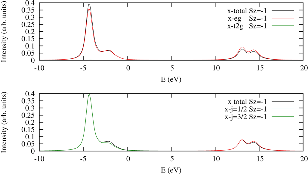 |
| $2p$ to $3d$ XAS Spectra. Top pannel decomposed into excitations into the $e_g$ or $t_{2g}$ orbitals. Bottom panel decomposed to excitations from the $2p_{j=1/2}$ or $2p_{j=3/2}$ orbitals. |
|---|
The output of the script is:
- XAS_partial.out
Start of BlockGroundState. Converge 3 states to an energy with relative variance smaller than  1.490116119384766E-06

Start of BlockOperatorPsiSerialRestricted
Outer loop   1, Number of Determinants:        45        45 last variance  2.335271462951932E+00
Start of BlockOperatorPsiSerialRestricted
Start of BlockGroundState. Converge 3 states to an energy with relative variance smaller than  1.490116119384766E-06

Start of BlockOperatorPsiSerial
 <E>    <S^2>  <L^2>  <J^2>  <S_z>  <L_z>  <l.s>  <F[2]> <F[4]> <Neg>  <Nt2g>
-2.882  1.999 12.000 15.052 -0.813 -0.234 -0.306 -1.020 -0.878  2.009  5.991
-2.721  1.999 12.000 15.142 -0.002 -0.001 -0.330 -1.020 -0.878  2.011  5.989
-2.560  1.999 12.000 15.211  0.810  0.233 -0.349 -1.020 -0.878  2.012  5.988
Start of LanczosTriDiagonalizeMC
Start of LanczosTriDiagonalizeMC
Start of LanczosTriDiagonalizeMC
Start of LanczosTriDiagonalizeMC
Start of LanczosTriDiagonalizeMC
Spectra printed to file: XASSpec.dat